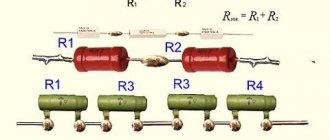
Loop inductance what is it, formula and calculation

Loop Inductance - Theory

Inductance is an idealized element whose properties are similar to an inductive coil, in which the energy of a magnetic field is accumulated.

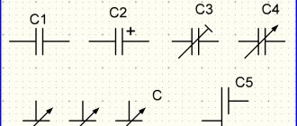
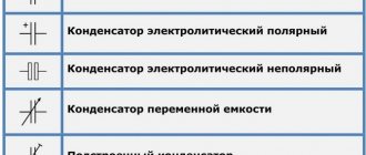
Symbol of inductance and positive directions of current, EMF of self-induction and voltage:

If a current is passed through a conductor, a magnetic flux Φ is created around it. The total magnetic flux (clutch flux) of the inductor is equal to Ψ= w×Φ, where Φ is the magnetic flux created by one turn; w is the number of turns.

By definition, self-inductance (or simply inductance) is equal to the proportionality coefficient between flux linkage and coil current L=Ψ/i.

Inductance is measured in Henry 1 H = 1 Wb / 1 A. The symbol L used to denote inductance was adopted in honor of Heinrich Friedrich Emil Lenz. The unit of inductance is named after Joseph Henry. The term inductance itself was coined by Oliver Heaviside in February 1886.

The coupling flux of the inductor is Ψ=L×i.

In accordance with the law of electromagnetic induction, when the magnetic flux changes in the coil, a self-inductive emf eL=-dΨ/dt is induced. The “-” sign is placed because the EMF has such a direction that the current it generates with its magnetic field prevents the change in the magnetic flux that causes this EMF.

The voltage across the inductance balances the EMF and can be written as uL=-eL=dΨ/dt=L×di/dt.

The instantaneous power entering the inductor is equal to p=uL×i=L×i×di/dt.

The energy stored in the inductor is wM=∫(0^t)ptd=∫(0^t)L×i×dt×di/dt=(L×i²)/2.

Mutual inductance characterizes the property of one element with current i1 to create a magnetic field that partially meshes with the turns w2 of another element.

The coefficient of mutual inductance is determined by the formula M=Ψ12/i2=Ψ21/i1, where Ψ12 is the coupling flux of the first circuit caused by the current of the second circuit (similar to Ψ21). Measured in Gn.

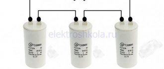
Capacitor in an electric current circuit

The principle of operation of a capacitor is simple - voltage is applied and a charge is accumulated. The drive behaves differently in two versions of the electrical circuit.

Permanent

If current is applied to a circuit with a capacitor connected to it, the needle on the ammeter will move, after which it will quickly return to its previous position. This is due to the fact that the device is charging quickly and the current has disappeared. Direct current cannot pass through plates separated by a dielectric. The practical use of a capacitor in such a circuit raises many questions. In direct current conditions, the capacitor functions, but for a short time. Transient processes in the form of charging and discharging remove all doubts. In DC electronic circuits, capacitors are one of the most common components.

Variable

When connecting alternating voltage, the poles of the capacitor change plus to minus with the frequency of the voltage supply. In this case, electrons move first to one and then to the other. During such a change, excess charge remains on the plates, which actually creates a current in the external circuit.

The capacitor in the AC circuit acts as a resistor.

Electromagnetic induction

Electromagnetic induction is the phenomenon of the occurrence of current in a closed conducting circuit when the magnetic flux passing through it changes.

The phenomenon of electromagnetic induction was discovered by Michael Faraday through a series of experiments.

Experience once. Two coils were wound on one non-conducting base in such a way that the turns of one coil were located between the turns of the second. The turns of the first coil were closed to a galvanometer, and the second were connected to a current source.

When the key was closed and current flowed through the second coil, a current pulse arose in the first. When the switch was opened, a current pulse was also observed, but the current through the galvanometer flowed in the opposite direction.

Experience two. The first coil was connected to a current source, and the second to a galvanometer. In this case, the second coil moved relative to the first. As the coil approached or moved away, the current was recorded.

Experience three. The coil was connected to a galvanometer, and the magnet was moved relative to the coil.

Here's what these experiments showed:

Induction current occurs only when the lines of magnetic induction change.

The direction of the current differs when the number of lines increases and when they decrease.

The strength of the induction current depends on the rate of change of the magnetic flux. In this case, both the field itself can change and the circuit can move in a non-uniform magnetic field.

Why does induced current occur?

Current in a circuit can exist when external forces act on free charges. The work done by these forces to move a single positive charge along a closed loop is equal to electromotive force (EMF).

This means that when the number of magnetic lines through the surface limited by the contour changes, an emf appears in it, which is called the induced emf.

Questions and tasks

Are the capacitances of two identical insulated conductors always the same?
Is it possible to charge a Leyden jar without grounding one of the plates?
What is approximately the electrical capacitance of your body?
Will the capacitance of a flat capacitor change if an uncharged thin metal plate is inserted into the air gap between its plates?
Find the capacitance of the system of capacitors connected between points A
and
B
, as shown in the figure.
The plates of a charged parallel-plate capacitor are alternately grounded. What will happen to the capacitor in this case?
A parallel-plate capacitor is connected to a source of constant emf. What needs to be done to create a magnetic field around the capacitor?
In the system shown in the figure, the outer sphere is connected to the ground once, and the inner one another time. Will the capacitance of such a capacitor be the same in these cases?
Why, if you turn on a capacitor in parallel with the switch, does the sparking stop when the switch opens?
A coil is wound tightly on top of the long solenoid. The current in the solenoid increases in direct proportion to time. What is the nature of the dependence of current on time in the coil?
A coil with a large number of turns was included in the city network. By measuring the alternating current flowing through the coil, it was determined that its resistance was 20 Ohms. Then they wound exactly the same second coil on top of this coil and connected it to the circuit parallel to the first. Will the total resistance of the coils be 10 ohms?
What happens if a transformer designed for an alternating voltage of the primary circuit of 127 V is connected to a DC network with a voltage of 110 V?
A collapsible school transformer, to the secondary winding of which a load is connected, is connected to the network. How will the current in the primary and secondary coils change when the top of the core is removed?
The oscillatory circuit consists of a capacitor of constant capacity and a coil into which the core can be inserted. One core is pressed from powdered magnetic iron compound (ferrite) and serves as an insulator. The other is made of copper. How will the natural frequency of the circuit change if a) a copper core, b) a ferrite core is inserted into the coil?
In the oscillatory circuit, the initial value of the charge on the capacitor was changed. Which characteristics of the electrical oscillations arising in the circuit will change as a result of this, and which will not?
What happens if a charged capacitor is connected by a superconductor to the same uncharged capacitor?
The flat capacitor included in the oscillatory circuit is such that its plates can move one relative to the other. How to “swing” the circuit by moving the plates?
The alternating current circuit consists of three series-connected resistances: ohmic, inductive and capacitive. Can a simultaneous increase in each of them lead to a decrease in overall resistance?
The circuit shown in the figure simultaneously transmits direct current and high frequency current. What needs to be done so that
only direct current passes
A
only high-frequency current passes B
The figure shows a section of an alternating current circuit. In what case does the voltage U
not depend on the current
I
?

How to find loop inductance

The formula, which is the simplest for finding the value, is the following:

L=F:I,

where F is the magnetic flux, I is the current in the circuit.

Self-inductive emf can be expressed through inductance:

Ei = -L x dI : dt.

The formula suggests a conclusion about the numerical equality of induction with EMF, which occurs in the circuit when the current changes by one ammeter in one second.

Variable inductance makes it possible to find the energy of the magnetic field:

W = L I2 : 2.

Answers

No, because in the presence of other conductors their capacitances may change.
It is impossible, since charges of both signs will arise on the insulated plate due to induction, and the bank will not be a capacitor.
In order of magnitude, the electrical capacitance of the human body is the same as the capacitance of a ball with a diameter of 1 m. It is approximately 50 pf.
Will not change.
Ctot
=
C
.
A capacitor with a capacitance C
0 is connected to points, the potential difference between which is zero.
Each of the plates has a certain, usually small, capacity relative to the ground. When the plate is grounded, part of the charge on it is neutralized. Therefore, the capacitor will discharge. But it will discharge the slower, the greater its capacity compared to the capacity of the plates relative to the ground.
In the first case, on a large sphere, charges will be located only on the inside. In the second case, they will be on both sides, and the capacitance of the entire capacitor will be equal to the capacitance of a system of two parallel-connected capacitors with plates AB
and
BC
(see figure).
It is necessary to bring the capacitor plates closer together or apart.
The self-induction current that occurs when the circuit is opened charges the capacitor and does not pass through the switch in the form of a spark.
If the coil is connected to a closed circuit, then a direct current will arise in it, the establishment time of which is determined by the inductance of the coil and its resistance.
After the second coil was wound on the first coil, the active resistance became half as large, but the inductive resistance remained the same. Consequently, the total resistance will decrease by less than half, i.e. it will be more than 10 ohms.
The transformer winding will burn out, since only its inductive resistance is high, while its active resistance is negligible.
By removing the top of the core, the inductances of the primary and secondary coils will decrease. This will lead to a decrease in the self-induced emf in the primary winding and the induced emf in the secondary. Consequently, the current in the primary coil will increase, and in the secondary coil it will decrease.
a) Foucault induction currents will arise in the copper core, the magnetic field of which will weaken the magnetic field of the coil. This will lead to a decrease in its inductance and, consequently, to an increase in the oscillation frequency, b) The ferrite core will increase the magnetic field of the coil, accordingly the inductance of the coil will increase, and the frequency will decrease.
The amplitudes of fluctuations in current, voltage, and magnetic induction will change; the period of oscillation will continue.
Undamped (if we neglect the radiation of electromagnetic waves) oscillations will arise in the system. Moreover, at the moment when the charge is distributed equally between the capacitors, the energy of the electrostatic field is minimal, and the energy of the magnetic field is maximum.
When the charge on the capacitor plates reaches its maximum value, the plates should be moved apart, and the work done will go to increase the energy of the circuit. When the charge is zero, the plates should be moved to their previous position - the energy in the circuit will not change.
Yes maybe.
An inductor must be connected
to branch A
a capacitor B.
If we neglect active resistance, then \(~U = I \left( \omega L - \frac{1}{\omega C}\right)\). Voltage does not depend on current only when \(~\omega L = \frac{1}{\omega C}\); in this case U

= 0 for any
I.

Necessary formulas for calculations

To find the inductance of the solenoid, the following formula is applied:

L= µ0n2V,

where µ0 shows the magnetic permeability of the vacuum, n is the number of turns, V is the volume of the solenoid.

You can also calculate the inductance of the solenoid using another formula:

L = µ0N2S : l,

It will be interesting➡ Determining the direction of the magnetic induction vector

where S is the cross-sectional area and l is the length of the solenoid.

To find the inductance of the solenoid, any formula is used that is suitable for solving the given problem.

Designation and units of measurement

Current resistance: formula

In honor of Lenz, the unit of inductance was designated by the symbol "L". Expressed as Henry, abbreviated as Gn (in English literature N), in honor of the famous American physicist.

Joseph Henry

If, with a current change of one ampere for every second, the self-inductive emf is 1 volt, then the inductance of the circuit will be measured in 1 henry.

How can inductance be designated in other systems:

In the SGS system, SGSM - in centimeters. To distinguish it from the unit of length, it is designated abhenry;
In the SGSE system - in StatHenry.

Properties

Has the following properties:

Depends on the number of turns of the circuit, its geometric dimensions and the magnetic properties of the core;
Cannot be negative;
Based on the definition, the rate of change of current in the circuit is limited by the value of its inductance;
As the frequency of the current increases, the reactance of the coil increases;
It has the property of storing energy - when the current is turned off, the stored energy tends to compensate for the drop in current.

Inductance and capacitor

The current-carrying elements of the device are capable of creating its own inductance. These are such structural parts as masonry, connecting busbars, down conductors, terminals and fuses. It is possible to create additional capacitor inductance by connecting busbars. The operating mode of an electrical circuit depends on inductance, capacitance and active resistance. The formula for calculating the inductance that occurs when approaching the resonant frequency is as follows:

Ce = C: (1 – 4Π2f2LC),

where Ce determines the effective capacitance of the capacitor, C indicates the actual capacitance, f is the frequency, L is the inductance.

The inductance value must always be taken into account when working with power capacitors. For pulse capacitors, the most important value is the self-inductance. Their discharge falls on the inductive circuit and has two types - aperiodic and oscillatory.

The inductance in a capacitor depends on the connection diagram of the elements in it. For example, when sections and buses are connected in parallel, this value is equal to the sum of the inductances of the package of main buses and terminals. To find this kind of inductance, the formula is as follows:

Lk = Lp + Lm + Lb,

where Lk shows the inductance of the device, Lp of the package, Lm of the main buses, and Lb of the inductance of the terminals.

If, in a parallel connection, the bus current varies along its length, then the equivalent inductance is determined as follows:

Lk = Lc : n + µ0 l x d : (3b) + Lb,

where l is the length of the tires, b is its width, and d is the distance between the tires.

To reduce the inductance of the device, it is necessary to arrange the current-carrying parts of the capacitor so that their magnetic fields are mutually compensated. In other words, current-carrying parts with the same current movement must be removed from each other as far as possible, and those with the opposite direction should be brought closer together. By combining down conductors with a decrease in dielectric thickness, the inductance of the section can be reduced. This can also be achieved by dividing one section with a large volume into several with smaller capacity.

Introduction

The frequency characteristics of capacitors are important parameters that are required for circuit design. Understanding the frequency characteristics of a capacitor will allow you to determine, for example, what noise a capacitor can suppress or what power supply voltage fluctuations it can control. This article describes two types of frequency responses: |Z| (impedance or total resistance) and ESR (capacitor equivalent series resistance).

The impedance Z of an ideal capacitor is given by formula 1, where ω is the angular frequency and C is the capacitance of the capacitor.

Figure 1. Ideal capacitor

(1)

From formula 1 it is clear that as the frequency increases, the impedance of the capacitor decreases. This is shown in Figure 1. In an ideal capacitor there is no loss and the equivalent series resistance (ESR) is zero.

Figure 2. Frequency response of an ideal capacitor

In a real capacitor (Fig. 3), there is some resistance (ESR) caused by dielectric losses, capacitor plate resistance losses and losses associated with leakage resistance, as well as parasitic inductance (ESL) of the capacitor leads and plates. As a result, the impedance frequency response takes on a V-shape (or U-shape depending on the type of capacitor), as shown in Figure 4. The figure also shows the ESR frequency response.

Figure 3. Real capacitor

Figure 4. Example of the frequency response of a real capacitor

The reason why graphs |Z| and ESR have the same form as in Figure 4, can be explained as follows. Low frequency region |Z| in this region decreases inversely with frequency, as in an ideal capacitor. The ESR value is determined by the dielectric loss in the capacitor. Resonance Region As the frequency increases, the ESR, as a result of stray inductance, electrode resistance and other factors, causes a deviation of |Z| from the ideal characteristic (red dotted line) and reaches the minimum value. The frequency at which |Z| reaches a minimum, is called the natural resonant frequency and at this frequency |Z| =ESR. After exceeding the natural resonance frequency, the element characteristic changes from capacitive to inductive and |Z| starts to rise. The region below the natural resonant frequency is called the capacitive region, and the region above is called the inductive region. In the resonance region, losses on the electrodes are added to the dielectric losses. High-frequency region With a further increase in frequency, the characteristic |Z| determined by the parasitic inductance of the capacitor. In the high-frequency region |Z| increases in proportion to frequency, according to formula 2. As for ESR, skin effect, proximity effect and others begin to appear in this area.

(2)

So, we looked at the frequency response of a real capacitor. The important thing to remember here is that as the frequency increases, ESR and ESL can no longer be ignored. Since there are a large number of applications in which capacitors are used at high frequencies, ESR and ESL become important parameters that characterize a capacitor in addition to its capacitance value.

The parasitic components of real capacitors have different meanings depending on their type. Let's look at the frequency characteristics of different capacitors. Figure 5 shows plots of |Z| and ESR for 10 µF capacitors. All capacitors, except film ones, are planar (SMD).

Figure 5. Frequency characteristics of different types of capacitors.

For all types of capacitors |Z| behaves the same up to 1 kHz. After 1 kHz, the impedance increases more strongly in aluminum and tantalum electrolytic capacitors than in monolithic ceramic and film capacitors. This is due to the fact that aluminum and tantalum capacitors have high electrolyte resistivity and high ESR. Film and monolithic ceramic capacitors use metal materials for the electrodes and hence have very low ESR. Monolithic ceramic capacitors and film capacitors show approximately the same characteristics up to the point of self-resonance, but monolithic ceramic capacitors have a higher resonant frequency and |Z| in the inductive region below. These results show that the impedance of SMD type monolithic ceramic capacitors is of small importance over a wide frequency range. This makes them most suitable for high frequency applications.

There are also several types of monolithic ceramic capacitors, made of different materials and having different shapes. Let's look at how these factors affect frequency response. ESR ESR in the capacitive region depends on the dielectric loss caused by the dielectric material. Class 2 dielectric materials based on ferroelectrics have a high dielectric constant and, as a rule, a high ESR. Class 1 materials - temperature-compensated materials based on paraelectrics - have low dielectric losses and low ESR. At high frequencies in the resonant and inductive regions, in addition to the resistance of the electrode material, their shape and the number of layers, the ESR depends on the skin effect and the proximity effect. Electrodes are often made of Ni, but for cheap capacitors Cu is sometimes used, which also has low resistance. ESL The ESL of monolithic ceramic capacitors is highly dependent on the internal structure of the electrodes. If the dimensions of the internal electrodes are given by length, width and thickness, then the inductance ESL can be determined mathematically. The ESL value decreases when the capacitor electrodes are shorter, wider and thinner. Figure 6 shows the relationship between the nominal capacitance and the resonant frequency of various types of monolithic ceramic capacitors. You can see that as the capacitor size decreases, the natural resonant frequency increases and the ESL decreases for the same capacitance values. This means that small capacitors with short lengths are better suited for high frequency applications.

Figure 6.

Figure 7 shows a reverse LW capacitor with short length L and large width W. From the frequency characteristics shown in Figure 8, it can be seen that the LW capacitor has lower impedance and better performance than a conventional capacitor of the same capacitance. With LW capacitors you can achieve the same performance as conventional capacitors, but with fewer components. Reducing the number of components reduces costs and reduces installation space.

Figure 7. External view of the reverse LW capacitor.

Figure 8. |Z| and ESR of reverse LW capacitor and general purpose capacitor

Based on materials from Murata. Free translation

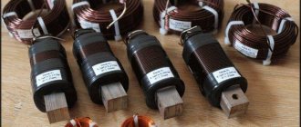
"Spool of thread"

An inductor is an insulated copper wire wound on a solid base. As for insulation, the choice of material is wide - varnish, wire insulation, and fabric. The magnitude of the magnetic flux depends on the area of the cylinder. If you increase the current in the coil, the magnetic field will become larger and vice versa.

If you apply an electric current to a coil, a voltage appears in it opposite to the current voltage, but it suddenly disappears. This kind of voltage is called electromotive force of self-induction. At the moment the voltage is turned on to the coil, the current changes its value from 0 to a certain number. The voltage at this moment also changes its value, according to Ohm’s law:

I = U : R,

where I characterizes the current strength, U indicates the voltage, R is the coil resistance.

Another special feature of the coil is the following fact: if you open the “coil - current source” circuit, the EMF will be added to the voltage. The current will also initially increase and then decline. This implies the first law of commutation, which states that the current strength in the inductor does not change instantly.

The coil can be divided into two types:

With magnetic tip. The material of the heart is ferrites and iron. The cores serve to increase inductance.
With non-magnetic. Used in cases where the inductance is no more than five milliHenry.

The devices differ in appearance and internal structure. Depending on these parameters, the inductance of the coil is determined. The formula is different in each case. For example, for a single-layer coil the inductance will be equal to:

L = 10µ0ΠN2R2 : 9R + 10l.

But for a multilayer one there is another formula:

L= µ0N2R2 :2Π(6R + 9l + 10w).

Main conclusions related to the operation of coils:

On a cylindrical ferrite, the largest inductance occurs in the middle.
To obtain maximum inductance, it is necessary to wind the turns closely on the coil.
The smaller the number of turns, the smaller the inductance.
In a toroidal core, the distance between the turns does not play the role of the coil.
The inductance value depends on the “turns squared”.
If inductances are connected in series, then their total value is equal to the sum of the inductances.
When connecting in parallel, you need to ensure that the inductances are spaced apart on the board. Otherwise, their readings will be incorrect due to the mutual influence of magnetic fields.

It will be interesting➡ Thermal relay for an electric motor

Series connection of a capacitor and an inductor. The concept of voltage resonance

General information

When the same sinusoidal current I flows through a circuit (Fig. 6.5.1) with a series connection of a capacitor and an inductor, the voltage across the capacitor UC lags the current I by 900, and the voltage across the inductor UL leads the current by 900. These voltages are in antiphase (rotated relative to each other by 1800).

Rice. 6.5.1

When one of the voltages is greater than the other, the circuit is either predominantly inductive (Fig. 6.5.2) or predominantly capacitive (Fig. 6.5.3). If the voltages UL and UC have the same values and compensate each other, then the total voltage in the L – C circuit section is equal to zero. Only a small voltage component remains at the active resistance of the coil and wires. This phenomenon is called stress resonance (Fig. 6.5.4).

Rice. 6.5.2

Rice. 6.5.3

Rice. 6.5.4

At voltage resonance, the reactance of the circuit

X = XL – XC

turns out to be zero. For given values of L and C, resonance can be obtained by changing the frequency.

Since XL = wL and XC = 1 / wC , then the resonant frequency w0 can be determined from the equation:

w0L – 1 / w0C = 0,

where

And .

The total resistance of the circuit at resonance turns out to be equal to the small active resistance of the coil, so the current in the circuit is in phase with the voltage and can be quite large even with a small applied voltage. In this case, the voltages UL and UC can significantly (tens of times!) exceed the applied voltage.

experimental part

Exercise

For a circuit with a series connection of a capacitor and an inductor, measure the effective values of the current I and voltages U , UC , UL at w = w0, w0 and w>w0. Construct vector diagrams.

Work order

· Assemble the circuit according to the diagram (Fig. 6.5.5), connect an adjustable sinusoidal voltage source and set the voltage at its input to 2 V and the frequency to 500 Hz. As an inductance with low active resistance, use a 300-turn transformer coil, inserting strips of paper in one layer (non-magnetic gap) between the horseshoes of the split core.

Rice. 6.5.5

· By changing the frequency of the applied voltage, achieve resonance at the maximum current. To fine-tune the maximum current, it is necessary to maintain a constant voltage at the input of the circuit. When measuring with virtual instruments, the resonance is adjusted by the transition through zero of the phase angle between the input voltage and current. There is then no need to keep the input voltage constant.

· Take measurements and record in the table. 6.5.1 measurement results at resonance f=f0 for f1 » 0.75 f0 and f2 » 1.25 f0.

Table 6.5.1

f, Hz	I, mA	U, B	UL,B	UC, B
f0 =
f1 =
f2 =

· Construct the vector diagrams in Fig. on the same scale. 6.5.6 for each of the considered cases.

Rice. 6.5.6

6.6. Parallel connection of a capacitor and an inductor. The concept of current resonance

General information

U is applied to a circuit (Fig. 6.6.1) with a parallel connection of a capacitor and an inductor , the same voltage is applied to both elements of the circuit.

Rice. 6.6.1

The total circuit current I branches into the current in the capacitor IC (the capacitive component of the total current) and the current in the coil IL (the inductive component of the total current), with the current IL lagging behind the voltage U by 900, and IC leading by 900.

Currents IC and IL have opposite phases (1800) and, depending on their values, balance each other completely or partially. They can be represented using vector current diagrams (Fig. 6.6.2 - 4).

When IC = IL current resonance occurs (vector diagram Fig. 6.6.2)

Rice. 6.6.2

Rice. 6.6.3

Rice. 6.6.4

When IC > IL, i.e. The capacitor current predominates, the total circuit current I is capacitive in nature and leads the voltage U by 900 (Fig. 6.6.3).

When IC < IL , i.e. the coil current prevails, the total circuit current I is inductive and lags behind the voltage U by 900 (Fig. 6.6.4).

These arguments were carried out neglecting the losses of active power in the capacitor and coil.

When currents resonate, the reactive conductivity of the circuit B = BL – BC is zero. The resonant frequency is determined from the equation

from where, just as with voltage resonance,

And .

The total conductivity at resonance of currents turns out to be close to zero. Only a small active conductivity remains uncompensated, due to the active resistance of the coil and imperfect insulation of the capacitor. Therefore, the current in the unbranched part of the circuit has a minimum value, while the currents IL and IC can exceed it tens of times.

experimental part

Exercise

For a circuit with a parallel connection of a capacitor and an inductor, measure the effective values of the voltage U and currents I, IC and IL at w = w0, w0 and w>w0. Construct vector diagrams.

Work order

· Assemble the circuit according to the diagram (Fig. 6.6.5), connect an adjustable sinusoidal voltage source and set its parameters: U = 7 V, f = 500 Hz. As an inductance with low active resistance, use a 300-turn transformer coil, inserting strips of paper in one layer (non-magnetic gap) between the horseshoes of the split core.

Rice. 6.6.5

· By changing the frequency of the applied voltage, achieve resonance at the minimum current I. For precise tuning, keep the circuit input voltage constant. When measuring with virtual instruments, the resonance is adjusted by the transition through zero of the phase angle between the input current and voltage. Then it is not necessary to maintain the voltage at the input of the circuit constant.

· Take measurements and record the measurement results in the table. 6.6.1 for f = f0 , f1 »0.75 f0 and f2 »1.25 f0 .

Table 6.6.1

f, Hz	U, B	I, mA	IL, mA	IC, mA
f0 =
f1 =
f2 =

· Construct the vector diagrams in Fig. on the same scale. 6.6.6 for each of the considered cases.

Rice. 6.6.6

6.7. Frequency characteristics of a series resonant circuit

General information

Frequency characteristics are usually called the dependences of the resistance and conductance of a circuit on the frequency of the sinusoidal applied voltage. Sometimes they also include dependences on the frequency of currents, voltages, phase shifts and powers.

In a series resonant circuit (Fig. 6.7.1a), active resistance does not depend on frequency, and inductive, capacitive and reactance change in accordance with the following expressions:

Rice. 6.7.1.

Total resistance, as follows from the resistance triangle (Fig. 6.7.1b):

The appearance of these frequency dependences is presented in Fig. 6.7.2a. At resonant frequency w0=1/√(LC):

XL(w0)=XC(w0)= √(L/C)=r

This resistance is called the characteristic impedance of the resonant circuit, and the ratio

r/R=Q

– quality factor of the resonant circuit

Figure 6.7.2b shows graphs of changes in current, voltage in sections of the circuit and phase shift with a change in frequency and a constant applied voltage in accordance with the following formulas:

I(w)=U/Z(w); UL(w)=wLI(w); UC=I/wC; φ=arctg[wL-1/(wCR)].

If Q>1, then at resonance the voltages UL(w0) and UC(w0) exceed the applied voltage by a factor of Q.

Rice.
6.7.2 When w0 the circuit is capacitive (the current leads the voltage by angle j), when w=w0 it is active, and when w>w0 it is inductive (the current lags behind the voltage).

experimental part

Exercise

Experimentally record the frequency characteristics of a series resonant circuit - R(w), X(w), Z(w), I(w), UL(w), UC(w) and j(w) - at Q >1.

Work order

Using an ohmmeter, measure the active resistance of the inductor shown in the diagram (Fig. 6.7.3).

R= Ohm.

· Calculate the resonant frequency, characteristic impedance and quality factor of the resonant circuit:

f0=1/2p√(LC)= Hz; r=√(L/C)= Ohm; Q=r/R= .

Assemble the circuit according to the diagram (Fig. 6.7.3), including the corresponding connector sockets as measuring instruments and considering the resistance R to be the resistance of the inductor. At this stage, take the additional resistance Rext equal to zero (Q>1). Connect an adjustable sinusoidal voltage source and set its parameters: U=5 V, f=f0.

Rice. 6.7.3.

Turn on the virtual devices and, based on the phase meter readings, adjust the resonant mode more accurately by changing the frequency of the applied voltage. Compare the experimental resonant frequency with the calculated one:

Experimental f0= Hz.

Calculated f0= Hz.

Changing the frequency from 0.2 to 2 kHz, write down the readings of virtual instruments in Table 6.7.1 and based on these results in Fig. 6.7.4. and 6.7.5. draw graphs of frequency characteristics for quality factor Q>1.
Include additional resistance Rext = 100...330 Ohm in the circuit and make sure that the resonant frequency has not changed, and the current and voltage UL and UC have become less at resonance.

Table 6.7.1.

f, Hz

R, Ohm

X, Ohm

Z, Ohm

I, mA

UC, V

URL, V

j, deg

6.8. Frequency characteristics of a parallel resonant circuit

General information

In a parallel resonant circuit (Fig. 6.8.1a), active conductivity does not depend on frequency, and inductive, capacitive and reactive conductances change in accordance with the following expressions:

BL(w)=1/ωL; BC(w)=ωC; B(w)= BL(w)- BC(w);

Rice. 6.8.1.

Total conductivity, as follows from the conductivity triangle (Fig. 6.8.1b):

Y(w)=√(G2+B2).

The appearance of these frequency dependences is presented in Fig. 6.8.2a.

At resonant frequency w0=1/√(LC):

BL(w0)=BC(w0)= √(C/L)=g .

This conductivity is called the characteristic conductance of the resonant circuit, and the ratio

g/G=Q

as well as in a series circuit - by quality factor.

When the frequency changes and the applied voltage remains constant, the currents change in proportion to the corresponding conductivities:

I(w)=UY(w); IL(w)=U/wL; IC=UwC, ILC=UB(w).

At the resonant frequency w=w0, the current I consumed from the source has a minimum and is equal to the current in the active resistance IR, and the current in the reactive section of the ILC circuit is zero (see Fig. 6.8.2a). Real curves may differ slightly from the ideal ones considered, since the active resistance of the coil was not taken into account here.

The phase shift angle (Fig. 6.8.2.b) changes in accordance with the expression:

φ=arctg[(1/wL-wC)/G].

When w0 the circuit is inductive (the current lags the voltage by angle j), when w=w0 it is active, and when w>w0 it is capacitive (the current leads the voltage). If Q>1, then at resonance the currents IL(w0) and IC(w0) exceed the source current I by Q times.

Rice. 6.8.2

In Fig. 6.8.2b, in addition to j(w), the dependences on the frequency of the total Z(w) and reactive X(w) resistances are also plotted. In the general case (see solid lines in the figure):

Z(w)=1/Y(w)=1/ √ (G2+B2);

X(w)=B/(G2+B2).

At resonance, the total resistance reaches its maximum value and the reactive value goes to zero.

In the idealized case, when the active conductance is so small that it can be neglected (G=0):

X(w)=1/B; Z(w)=1/|B|.

Then at the resonance point the curves X(w) and Z(w) have a discontinuity (see dotted lines in Fig. 6.8.2b).

experimental part

Exercise

Experimentally measure the frequency characteristics of a parallel resonant circuit with a high quality factor - I(w), IL(w), IC(w), X(w), Z(w) and j(w).

Work order

Assemble the circuit according to the diagram (Fig. 6.8.3), including measuring instruments or corresponding connector sockets. As an inductor with low active resistance, use the transformer winding W = 300 turns, inserting strips of paper in one layer between the horseshoes of the detachable core.

· Apply a sinusoidal voltage to the circuit from a voltage generator of a special form U=5B, f=500Hz.

· Measure the reactance of the inductor using virtual instruments or calculate the reactance of the inductor using the readings of multimeters and calculate the inductance and resonant frequency:

XL=U/IL= Ohm;

L= XL/(2pf)= Gn;

f0=1/2p√(LC)= Hz.

Rice. 6.8.3.

Based on the phase meter reading or the minimum current I, adjust the resonant mode by changing the frequency of the applied voltage. Compare the experimental resonant frequency with the calculated one:

Experimental f0= Hz.

Calculated f0= Hz.

Changing the frequency from 0.2 to 1 kHz, write down the readings of virtual instruments in Table 6.8.1 and based on these results in Fig. 6.8.4. and 6.8.5. draw frequency response graphs.

Notes:

1. If there are no virtual instruments, write down the currents measured by multimeters in the table, and calculate the resistances using the formulas given in the “General Information” section. In this case, the phase shift can be determined from vector diagrams constructed for each frequency value.

2. In the region of the resonant frequency, the experimental points should be located more densely than at the edges of the graphs.

f, Hz

X, Ohm

Z, Ohm

I, mA

IC, mA

IL, mA

j, deg

Table 6.7.1.

General information

Rice. 6.5.1

Rice. 6.5.2

Rice. 6.5.3

Rice. 6.5.4

At voltage resonance, the reactance of the circuit

X = XL – XC

turns out to be zero. For given values of L and C, resonance can be obtained by changing the frequency.

Since XL = wL and XC = 1 / wC , then the resonant frequency w0 can be determined from the equation:

w0L – 1 / w0C = 0,

where

And .

experimental part

Exercise

For a circuit with a series connection of a capacitor and an inductor, measure the effective values of the current I and voltages U , UC , UL at w = w0, w0 and w>w0. Construct vector diagrams.

Work order

Rice. 6.5.5

· Take measurements and record in the table. 6.5.1 measurement results at resonance f=f0 for f1 » 0.75 f0 and f2 » 1.25 f0.

Table 6.5.1

f, Hz	I, mA	U, B	UL,B	UC, B
f0 =
f1 =
f2 =

· Construct the vector diagrams in Fig. on the same scale. 6.5.6 for each of the considered cases.

Rice. 6.5.6

6.6. Parallel connection of a capacitor and an inductor. The concept of current resonance

General information

U is applied to a circuit (Fig. 6.6.1) with a parallel connection of a capacitor and an inductor , the same voltage is applied to both elements of the circuit.

Rice. 6.6.1

Currents IC and IL have opposite phases (1800) and, depending on their values, balance each other completely or partially. They can be represented using vector current diagrams (Fig. 6.6.2 - 4).

When IC = IL current resonance occurs (vector diagram Fig. 6.6.2)

Rice. 6.6.2

Rice. 6.6.3

Rice. 6.6.4

When IC > IL, i.e. The capacitor current predominates, the total circuit current I is capacitive in nature and leads the voltage U by 900 (Fig. 6.6.3).

When IC < IL , i.e. the coil current prevails, the total circuit current I is inductive and lags behind the voltage U by 900 (Fig. 6.6.4).

These arguments were carried out neglecting the losses of active power in the capacitor and coil.

When currents resonate, the reactive conductivity of the circuit B = BL – BC is zero. The resonant frequency is determined from the equation

from where, just as with voltage resonance,

And .

experimental part

Exercise

Work order

Rice. 6.6.5

· Take measurements and record the measurement results in the table. 6.6.1 for f = f0 , f1 »0.75 f0 and f2 »1.25 f0 .

Table 6.6.1

f, Hz	U, B	I, mA	IL, mA	IC, mA
f0 =
f1 =
f2 =

· Construct the vector diagrams in Fig. on the same scale. 6.6.6 for each of the considered cases.

Rice. 6.6.6

6.7. Frequency characteristics of a series resonant circuit

General information

In a series resonant circuit (Fig. 6.7.1a), active resistance does not depend on frequency, and inductive, capacitive and reactance change in accordance with the following expressions:

Rice. 6.7.1.

Total resistance, as follows from the resistance triangle (Fig. 6.7.1b):

The appearance of these frequency dependences is presented in Fig. 6.7.2a. At resonant frequency w0=1/√(LC):

XL(w0)=XC(w0)= √(L/C)=r

This resistance is called the characteristic impedance of the resonant circuit, and the ratio

r/R=Q

– quality factor of the resonant circuit

I(w)=U/Z(w); UL(w)=wLI(w); UC=I/wC; φ=arctg[wL-1/(wCR)].

If Q>1, then at resonance the voltages UL(w0) and UC(w0) exceed the applied voltage by a factor of Q.

Rice.
6.7.2 When w0 the circuit is capacitive (the current leads the voltage by angle j), when w=w0 it is active, and when w>w0 it is inductive (the current lags behind the voltage).

experimental part

Exercise

Experimentally record the frequency characteristics of a series resonant circuit - R(w), X(w), Z(w), I(w), UL(w), UC(w) and j(w) - at Q >1.

Work order

Using an ohmmeter, measure the active resistance of the inductor shown in the diagram (Fig. 6.7.3).

R= Ohm.

· Calculate the resonant frequency, characteristic impedance and quality factor of the resonant circuit:

f0=1/2p√(LC)= Hz; r=√(L/C)= Ohm; Q=r/R= .

Assemble the circuit according to the diagram (Fig. 6.7.3), including the corresponding connector sockets as measuring instruments and considering the resistance R to be the resistance of the inductor. At this stage, take the additional resistance Rext equal to zero (Q>1). Connect an adjustable sinusoidal voltage source and set its parameters: U=5 V, f=f0.

Rice. 6.7.3.

Turn on the virtual devices and, based on the phase meter readings, adjust the resonant mode more accurately by changing the frequency of the applied voltage. Compare the experimental resonant frequency with the calculated one:

Experimental f0= Hz.

Calculated f0= Hz.

Changing the frequency from 0.2 to 2 kHz, write down the readings of virtual instruments in Table 6.7.1 and based on these results in Fig. 6.7.4. and 6.7.5. draw graphs of frequency characteristics for quality factor Q>1.
Include additional resistance Rext = 100...330 Ohm in the circuit and make sure that the resonant frequency has not changed, and the current and voltage UL and UC have become less at resonance.

Table 6.7.1.

f, Hz

R, Ohm

X, Ohm

Z, Ohm

I, mA

UC, V

URL, V

j, deg

6.8. Frequency characteristics of a parallel resonant circuit

General information

BL(w)=1/ωL; BC(w)=ωC; B(w)= BL(w)- BC(w);

Rice. 6.8.1.

Total conductivity, as follows from the conductivity triangle (Fig. 6.8.1b):

Y(w)=√(G2+B2).

The appearance of these frequency dependences is presented in Fig. 6.8.2a.

At resonant frequency w0=1/√(LC):

BL(w0)=BC(w0)= √(C/L)=g .

This conductivity is called the characteristic conductance of the resonant circuit, and the ratio

g/G=Q

as well as in a series circuit - by quality factor.

When the frequency changes and the applied voltage remains constant, the currents change in proportion to the corresponding conductivities:

I(w)=UY(w); IL(w)=U/wL; IC=UwC, ILC=UB(w).

The phase shift angle (Fig. 6.8.2.b) changes in accordance with the expression:

φ=arctg[(1/wL-wC)/G].

Rice. 6.8.2

In Fig. 6.8.2b, in addition to j(w), the dependences on the frequency of the total Z(w) and reactive X(w) resistances are also plotted. In the general case (see solid lines in the figure):

Z(w)=1/Y(w)=1/ √ (G2+B2);

X(w)=B/(G2+B2).

At resonance, the total resistance reaches its maximum value and the reactive value goes to zero.

In the idealized case, when the active conductance is so small that it can be neglected (G=0):

X(w)=1/B; Z(w)=1/|B|.

Then at the resonance point the curves X(w) and Z(w) have a discontinuity (see dotted lines in Fig. 6.8.2b).

experimental part

Exercise

Experimentally measure the frequency characteristics of a parallel resonant circuit with a high quality factor - I(w), IL(w), IC(w), X(w), Z(w) and j(w).

Work order

Assemble the circuit according to the diagram (Fig. 6.8.3), including measuring instruments or corresponding connector sockets. As an inductor with low active resistance, use the transformer winding W = 300 turns, inserting strips of paper in one layer between the horseshoes of the detachable core.

· Apply a sinusoidal voltage to the circuit from a voltage generator of a special form U=5B, f=500Hz.

· Measure the reactance of the inductor using virtual instruments or calculate the reactance of the inductor using the readings of multimeters and calculate the inductance and resonant frequency:

XL=U/IL= Ohm;

L= XL/(2pf)= Gn;

f0=1/2p√(LC)= Hz.

Rice. 6.8.3.

Based on the phase meter reading or the minimum current I, adjust the resonant mode by changing the frequency of the applied voltage. Compare the experimental resonant frequency with the calculated one:

Experimental f0= Hz.

Calculated f0= Hz.

Changing the frequency from 0.2 to 1 kHz, write down the readings of virtual instruments in Table 6.8.1 and based on these results in Fig. 6.8.4. and 6.8.5. draw frequency response graphs.

Notes:

2. In the region of the resonant frequency, the experimental points should be located more densely than at the edges of the graphs.

f, Hz

X, Ohm

Z, Ohm

I, mA

IC, mA

IL, mA

j, deg

Table 6.7.1.

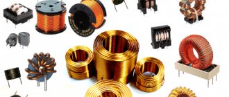
Application of inductors

Inductors are widely used in analog and signal processing circuits. They combine with capacitors and other radio components to form special circuits that can amplify or filter signals of a specific frequency.

Inductors have a wide range of applications ranging from large inductors such as power supply chokes that, in combination with filter capacitors, eliminate residual noise and other oscillations in the power supply output, to as small inductors as those found inside integrated circuits.

Two (or more) inductors, which are connected by a single magnetic flux, form a transformer, which is the main component of circuits operating with an electrical power supply network. Transformer efficiency increases with increasing voltage frequency.

For this reason, aircraft use AC voltage with a frequency of 400 hertz instead of the usual 50 or 60 hertz, which in turn allows for significant savings in the mass of transformers used in the aircraft power supply.

Inductors are also used as energy storage devices in switching voltage stabilizers, in high-voltage electrical power transmission systems to deliberately reduce system voltage or limit short-circuit current.

Ceramic capacitors

Types and properties of ceramics

This type of capacitor refers to capacitors with an inorganic dielectric. Ceramic capacitors are the most popular type of capacitors, due to their high and stable characteristics, ease of production, and suitability for automated installation [1]. Ceramic capacitors get their name because they use radio frequency ceramics based on titanium, zirconium and oxides of other materials as a dielectric. Most commonly, RF ceramics are made from titanium dioxide (TiO2), barium titanate (BaTiO3), or strontium titanate (SrTiO3), although the exact ceramic formulas vary between manufacturers.

Now it is necessary to say a few words about the classification of ceramic capacitors. Quite often, the “ultimate goal” of a review article on electronic components is an attempt to provide the developer with a universal tool for selecting components for use in a specific application, based on classification according to various parameters. In relation to ceramic capacitors, attempts to create a classification “to help the developer” must be considered rather unsuccessful. There is more than one reason for this, and the bottom line is that it would be more correct to admit that the most reliable way to select ceramic capacitors for a specific application is to read the datasheet.

Suffice it to mention that two engineering communities have proposed their own versions of the classification: IEC (International Electrotechnical Commissiom) and EIA (Electronic Industries Alliance). Classifications have differences. Thus, the EIA divides ceramics into four classes, and the IEC into three. The fact that a significant portion of manufacturers (mostly American) use the EIA classification to label their products, while others use the IEC classification, only complicates the task of selecting components. It should be added here that the IEC encoding is also called Industrial, although in essence both encodings operate in the industrial temperature range. There is also a separate Military encoding. This section of the article will mainly refer to EIA and Industrial encodings.

There have been attempts at classification based on the division of capacitors by application, in which, however, it can be seen that the division by application is predominantly related to frequency. The same EIA proposes dividing ceramic capacitors into two large classes. One can rather roughly distinguish between higher-frequency applications (resonant circuits, etc. equipment), where low losses and high capacitance stability are of considerable importance, and less high-frequency applications (filtering circuits, etc.), where these parameters are not so significant ([1] , EIA).

Ceramic capacitors are capacitors with a standardized TKE value. As mentioned, the Electronics Industry Association (EIA) divides ceramics into four classes and types within each class. The lower the class number, the higher the overall performance of the capacitor, but the larger the size for a given capacitance. The types within each class define the recommended operating temperature range and TKE, including temperature drift and tolerance in said temperature drift. EIA defines the basic parameters of capacitors for each class and methods for measuring them. This applies to insulation resistance, dielectric loss tangent, dielectric absorption and other basic parameters of capacitors.

The division of ceramic capacitors into classes is quite arbitrary, since strict requirements for each class are not specified.
For example, class 1 capacitors are considered to be “precise temperature-compensated capacitors with high stability in voltage, temperature and frequency.” Class 1 capacitors are characterized by a temperature coefficient of no worse than ±3% per degree at +25…+85 °C. For Class 1 capacitors, an accuracy of 1% can be achieved, although an accuracy of 5–10% is considered most typical. The temperature dependence of capacitance for class 1 capacitors is considered linear. Ceramic capacitors are divided into classes according to the type of ceramic used in their manufacture. The EIA has introduced a set of codes to identify ceramic types. The codes for class 1 and class 2 ceramic capacitors are different. In addition, there are two options for designating the type of ceramic - in accordance with the EIA-RS‑198 standard and the Industrial standard mentioned above. Table 1 shows the EIA coding for Class 1 ceramics. Table 1. EIA-RS‑198 coding of ceramics according to the slope of the temperature curve (class 1)

Temperature coefficient (slope of temperature curve)		Temperature coefficient multiplier		Permissible temperature coefficient deviation, +25… +85 °C
Letter	ppm/°С	Number	Factor	Letter	ppm/°С
C	0	0	–1	G	±30
B	0,3	1	–10	H	±60
L	0,8	2	–100	J	±120
A	0,9	3	–1000	K	±250
M	1	4	+1	L	±500
P	1,5	6	+10	M	±1000
R	2,2	7	+100	N	±2500
S	3,3	8	+1000
T	4,7
V	5,6
U	7,5

For example, C0G ceramics are most often used in class 1 capacitors.
This means that in the temperature range of +25...+85 °C the slope of the temperature curve will be zero (0), that is, there will be no dependence of the capacitance on temperature. This can be seen in Fig. 1, 2, where the C0G capacitors are designated NP0 (the designation used in the Industrial standard). The temperature coefficient multiplier, together with the coefficient itself, also determines the slope of the temperature curve and, accordingly, the degree of change in capacitance due to temperature variations. In our example (C0G), a coefficient of 1 will not change the slope of the temperature curve specified by the main temperature coefficient (0), which in English literature is often called Significant Figures. The sign in front of the temperature coefficient multiplier determines the direction of change in capacitance: the “–” sign indicates that with increasing temperature the capacitance will decrease. The effect of the sign on the temperature coefficient multiplier is clearly demonstrated in Fig. 1. An explanation needs to be made for the drawing. The ceramic industry designation, based on the Negativ/Positive designation, is considered more outdated than the EIA designation, but is more intuitive and consists of a letter (N for negative temperature coefficient, P for positive temperature coefficient) and a number , indicating the temperature error. A comparison of EIA and industrial encoding can be seen in Table 2. Table 2. Comparative EIA and Industrial encoding

Industry	P100	NP0	N030	N075	N150	N220	N330	N470	N750	N1500	N2200
EIA	M7G	C0G	B2G	U1G	P2G	R2G	S2H	T2H	U2J	P3K

Now, actually, fig. 1, which was mentioned above. It shows the change in capacity as a function of temperature for class 1 ceramics. The various ceramic materials in this figure are Industrial coded (colored) and can be found in Table 2 to match their EIA codes (black boxed symbols). When comparing tables 1 and 2, one can see the effect of the sign of the temperature coefficient multiplier, illustrated in Fig. 1.

Rice. 1. Idealized curves of the dependence of capacity on temperature of class 1 ceramics

The main difference between class 2 ceramics and class 1 is the nonlinear dependence of capacity on temperature. This is clearly visible in Fig. 2, which compares ceramics of the 1st class C0G (NP0) with two samples of the 2nd class (X7R, Y5V). In general, class 2 capacitors have greater volumetric efficiency, which is associated with the high dielectric constant of class 2 ceramics and is directly reflected in the size of the capacitors.

Rice. 2. Comparison of the temperature characteristics of ceramics of the 1st and 2nd classes

The EIA temperature coding for Class 2 capacitors is shown in Table 3.
Table 3. EIA-RS-198 coding for ceramics without temperature compensation (Class 2 and higher)

Lowest operating temperature		Highest operating temperature		Changing Capacity
Letter	Temperature, °C	Number	Temperature, °C	Letter	V %
X	–55	4	+65	A	±1
Y	–30	5	+85	B	±1,5
Z	+10	6	+105	C	±2,2
7	+125	D	±3,3
8	+150	E	±4,7
9	+200	F	±7,5
P	±10
R	±15
S	±22
T	+22/–33
U	+22/–56
V	+22/–82

In addition to the temperature dependence described above, class 2 ceramics also have a clear dependence of capacitance on the applied constant or slowly varying voltage. The essence of this phenomenon is that when a constant voltage is applied to ferroelectrics used as ceramics in class 2 capacitors, the dielectric constant decreases due to polarization effects. As a consequence, the capacitance associated with the dielectric constant decreases. In English-language documentation, this phenomenon is often described by the term DC-bias (direct current bias).

This property is almost never mentioned when trying to classify capacitors, and specific values for the change in capacitance can be obtained mainly by studying the technical documentation for a specific product.

It should also be noted that a significant contribution to the description of this phenomenon was made by employees of the Japanese company Murata. They conducted research on domain structures of ceramics and proposed interactive software for hardware engineers to take DC bias into account when designing. In Fig. 3 you can see an example from Murata - here is the dependence of capacitance on DC voltage for class 2 ceramic capacitors (X5R, X7R).

Rice. 3. An example of the dependence of the capacitance of ceramics X5R, X7R on the applied constant voltage (Murata)

The direct correspondence between the type of ceramic and the frequency range is indicated in the technical documentation for a particular capacitor.
It is believed that class 1 capacitors are higher frequency and have the lowest losses and the least dissipation in the upper high-frequency range. Nevertheless, class 1 capacitors have a direct relationship between the maximum operating frequency and the capacitor rating. This can be seen in Table 4 when comparing the two types of ceramics in the frequency domain. Table 4. Comparison of ceramics of 1st and 2nd classes

10 pF	100 pF	1 nF	10 nF	100 nF	1 µF
C0G (class 1)	1550 MHz	460 MHz	160 MHz	55 MHz
X7R (Class 2)	190 MHz	56 MHz	22 MHz	10 MHz

And it should be borne in mind that dielectrics of the 2nd, 3rd and 4th classes are piezoelectrics, and therefore capacitors of these classes are susceptible to the microphone effect. This must be taken into account when deciding on the use of capacitors of these classes at frequencies above 200 MHz. But when such capacitors are used in power supplies, even pulsed ones, the microphone effect does not appear so clearly, except when the operating frequency is in the audio range. The influence of the piezoelectric effect on ceramics of the 2nd class is less than on ceramics of the 3rd and 4th classes. The presence of the piezoelectric effect in most types of ceramics used in the production of ceramic capacitors requires, when designing electrical circuits with ceramic capacitors, mandatory consideration of the reactive power dissipated by the capacitors, since in conditions when the reactive power is equal to or exceeds the active power dissipated by the capacitors, rapid aging occurs ceramics with its subsequent destruction. This is especially important when ceramic capacitors are used in power or filter circuits, such as power supply circuits for computer processors.

In addition to classification by type of ceramic, ceramic capacitors are ranked by design. The following groups of ceramic capacitors are distinguished:

polymer-coated disk capacitors for printed circuit mounting (disk);
single layer ceramic capacitors (single layer);
multilayer rectangular capacitors for surface mounting (multilayer);
packageless disk capacitors for surface mounting for use in the UHF range (decimeter wave range);
Tubular capacitors for printed circuit mounting are currently used extremely rarely.

Single Layer Ceramic Capacitor (SLCC)

In the class of ceramic capacitors, the type of so-called single-layer, or monolithic, capacitors should be noted.

Because SLCC uses the same ceramics, conductive materials, and many of the same technologies as multilayer capacitors, there are significant similarities in the temperature and frequency properties of MLCC and SLCC.

Single-layer ceramic capacitors are in some ways an elementary classical capacitor, since their design consists of two electrodes, between which a layer of high-frequency ceramics is located (Fig. 4).

Rice. 4. Dielectric Laboratories Single Layer Capacitor Design

Capacitors of this type are produced using the technology of sintering dissimilar materials and are, in fact, a ceramic-metal composite alloy. Therefore, they are intended primarily for use in integrated assemblies, including microwave ones. Although some manufacturers, for example Vishay, use the same technology to produce disk capacitors (Disk) for printed circuit mounting. The undoubted advantages of single-layer monolithic capacitors include:

very low transmission losses and low scattering at frequencies up to 50 GHz;
operating frequency range: up to 100 GHz;
reliable and durable design, including resistance to fracture;
nominal capacitance: 0.04–6200 pF;
dielectric constant of ceramics: 14–25000;
operating voltage: up to 100 V.

Classification of single-layer capacitors

There are several options for classifying single-layer capacitors. One of them is used by Dielectric Laboratories. It includes the following types:

Border Caps are conventional flat-plate broadband capacitors with reduced metallization on one or two sides. Reducing the metallization area helps prevent shorting of the plates during installation and improves visual inspection. The appearance and types of such capacitors are shown in Fig. 4.
Di-Cap are ordinary flat-plate broadband capacitors, the metallization area of which is equal to the area of the ceramic. Used in the frequency range 100 kHz – 80 GHz. The same type of capacitors can be output (Fig. 5).
Gap Cap - two series-connected capacitors on one ceramic plate (Fig. 6). Capacitors of this type can be connected in series to a microstrip line without the use of conductors.
Bar Cap1—capacitor assemblies. The main range of applications is up to 30 GHz. Manufactured for use, inter alia, in monolithic microwave integrated circuits (MMIC), Fig. 7.
Bi-Cap (Binary-Cap) - several capacitors on one ceramic plate. Capacities are related as powers of two. The main range of applications is up to 30 GHz. Used for prototyping and fine-tuning circuits. They have dimensions comparable to the geometry of components used in microwave devices. Capacitors on one plate can be used either singly or in combination (Fig. 8).
T‑Cap is a series of capacitors similar to Di-Cap. Has a different size range.
Milli-Cap - surface mount capacitors.

Rice. 5. Di-Cap Lead Capacitors from Dielectric Laboratories

Rice. 6. Gap-Cap by Dielectric Laboratories

Rice. 7. Bar-Cap by Dielectric Laboratories

Rice. 8. Bi-Cap from Dielectric Laboratories

Of interest is the comparative frequency response of several types of single-layer capacitors, shown in Fig. 9. Next, a similar diagram will be presented for multilayer capacitors.

Rice. 9. Comparative frequency response of different types of single-layer capacitors

Application of SLCC

Due to the low capacitance values due to the design of the classic single-layer capacitor and the outstanding frequency properties of ceramics, SLCCs have become most widespread in high-frequency and microwave applications. The use of ceramic types with high dielectric constants allows us to support the trend towards permanent miniaturization of this class of capacitors. A clear illustration of this can be found in the materials of the AVX company [2] (Fig. 10).

Rice. 10. Miniaturization of SLCC [1]

A typical example of properties that meet modern requirements for microwave components can be considered a series of ultra-wideband blocking single-layer ceramic capacitors GX from AVX [2]. The products are characterized by ultra-low insertion loss and low return loss. They are used in the frequency range up to 40 GHz and voltages up to 50 V, have capacitances up to 100 nF and form factor 0603-0201. In Fig. Figure 11 shows a typical insertion loss graph for the GX0S series.

Rice. 11. Insertion loss (S21) for GX0S (AVX) series blocking capacitors

General information

In order to understand what the inductance of the coil depends on, it is necessary to study in detail all the information about this physical quantity. The first step is to consider the accepted international designation of the parameter, its purpose, characteristics and units of measurement.

The very concept of inductance was proposed by the famous English physicist Oliver Heaviside, who studied it. This scientist gave the world other well-known terms - electrical conductivity, magnetic permeability and resistance, as well as EMF (electromotive force).

The first letter of the surname of another famous physicist, Emilia Lenza, was taken as a designation for inductance in formulas and when carrying out calculations. Today, the symbol L continues to be used when referring to this parameter.

The outstanding American physicist Joseph Henry was the first to discover the phenomenon of inductance. In his honor, physicists named the unit of measurement in the international SI, which is most often used in calculations. In other systems (Gaussian and SGS), inductance is measured in centimeters. To simplify the calculations, a relationship was adopted in which 1 cm equals 1 nanohenry. The very rarely used SGSE system leaves the self-induction coefficient without any units of measurement or uses the stathenry value. It depends on several parameters and is approximately equal to 89875520000 henry.

Among the main properties of inductance are:

The parameter value can never be less than zero.
The indicator depends only on the magnetic properties of the coil core, as well as on the geometric dimensions of the circuit.

Real capacitor parameters

I think you all know that there is nothing ideal in our reckless world. The same goes for electronics. Radio elements, cascades, radio nodes also often fail. You can even recall the recent story with the Progress spacecraft. The failure of some component led to the death of an entire giant in the space industry. Even a seemingly simple radio element, a capacitor, contains not only capacitance, but also other parasitic parameters. Let's look at the circuit, what does our real capacitor consist of?

Where

r is the resistance of the dielectric and the housing between the capacitor plates

C is the actual capacitance of the capacitor

ESR - equivalent series resistance

ESI (more often called ESL) - equivalent series inductance

This is actually what a simple harmless capacitor, especially an electrolytic one, consists of. Let's look at these parameters in more detail:

r is the dielectric resistance. The dielectric can be the electrolyte in electrolytic capacitors, paper or some other crap). Also between the terminals of the capacitor is its body. It also has some kind of resistance and is also made of dielectric and belongs here.

C is the capacitance of the capacitor, which is written on the capacitor itself, plus or minus some deviations associated with the error.

ESI(ESL) - series inductance is the self-inductance of the plates and leads. At low frequencies it can be ignored. Why? Read the article: inductor in direct and alternating current circuits.

Calculation methods

There are several basic ways to determine the inductance of a coil. All formulas that will be used in the calculations can be easily found in reference books or on the Internet. The whole calculation process is quite simple and will not be difficult for people with basic mathematical and physical knowledge.

Through current

This calculation is considered the simplest way to determine the inductance of a coil. The formula through current follows from the term itself. What is the inductance of the coil can be determined by the formula: L=Ф/I, where:

L - circuit inductance (in Henry);
F is the magnitude of the magnetic flux, measured in webers;
I is the current strength in the coil (in amperes).

This formula is only suitable for a single-turn circuit. If the coil consists of several turns, then instead of the magnetic flux value, the total flux (total value) is used. When the same magnetic flux passes through all the turns, then to determine the total value it is enough to multiply the value of one of them by the total number.

Finite Length Solenoid

The solenoid is a thin long coil, where the thickness of the winding is significantly less than the diameter. In this case, calculations are carried out using the same formula as through current strength, only the magnitude of the magnetic flux will be determined as follows: Ф=µ0NS/l, where:

µ0 is the magnetic permeability of the medium, determined from lookup tables (for air, which is taken by default in most calculations, it is equal to 0.00000126 henry/meter);
N is the number of turns in the coil;
S is the cross-sectional area of the coil, measured in square meters;
l is the length of the solenoid in meters.

The self-induction coefficient of the solenoid can also be calculated based on the method for determining the energy of the magnetic flux of the field. This is a simpler option, but it requires some quantities. The formula for finding inductance is L=2W/I 2, where:

W is the magnetic flux energy, measured in joules;
I is the current strength in amperes.

Toroidal core coil

In most cases, the toroidal coil is wound on a core made of a material with high magnetic permeability. In this case, to calculate the inductance, you can use the formula for a straight solenoid of infinite length. It has the following form: L=N µ0 µS/2 πr, where:

N is the number of coil turns;
µ—relative magnetic permeability;
µ0—magnetic constant;
S is the cross-sectional area of the core;
π is a mathematical constant equal to 3.14;
r is the average radius of the torus.

It will be interesting➡ Features of using pass-through switches

Long conductor

Most of these quasi-linear conductors have a circular cross-section. In this case, the value of the self-induction coefficient will be determined by the standard formula for approximate calculations: L= µ0l (µelnl/r+ µi/4)/2 π. The following notations are used here:

l is the length of the conductor in meters;
r is the radius of the wire cross-section, measured in meters;
µ0—magnetic constant;
µi is the relative magnetic permeability characteristic of the material from which the conductor is made;
µe is the relative magnetic permeability of the external environment (most often the value for vacuum is taken to be 1);
π—pi number;
ln is the notation for logarithm.

Why is a high ESR value harmful?

Previously, even when the first electronic circuits had just begun to appear, such a parameter as ESR was not even heard of by anyone. Maybe they knew that there was this resistance, but it did not harm anyone. But... with the advent of the first switching power supplies, people began to talk more and more often about ESR. Why did switching power supplies not like such harmless resistance?

At zero frequency (direct current) and low frequencies, as you remember from the article capacitor in a direct and alternating current circuit, the capacitor itself provides great resistance to electric current. In this case, some parasitic Ohm fractions of the ESR resistance will not affect the parameters of the electrical circuit. All the fun begins when the capacitor operates in high-frequency (HF) circuits.

You and I know that a capacitor passes alternating current through itself. And the higher the frequency, the lower the resistance of the capacitor itself. Here's the formula in case you forgot:

where XC is the resistance of the capacitor, Ohm

P is a constant and equals approximately 3.14

F - frequency, measured in Hertz

C - capacitance, measured in Farads

But we didn’t take one thing into account... The resistance of the leads and plates does not change with frequency! So... and if you think about it, it turns out that at an infinite frequency the resistance of the capacitor will be equal to its ESR? It turns out that our capacitor turns into a resistor? How does a resistor behave in an AC circuit? Yes, just like in a DC circuit: it gets hot! Therefore, this resistor will dissipate power P into the environment. And as you remember, power through resistance and current is expressed by the formula:

P=I2xR

Where

I is the current strength, in Amperes

R - ESR resistor resistance, in Ohms

This means that if the ESR is greater, then the power dissipation will also be greater! That is, this resistor will heat up quite well.

Are you catching up on what I’m telling you?

From all of the above, we can draw a simple conclusion: a capacitor with a large ESR in high-frequency circuits with high currents will heat up. Well, okay, let it warm up... Resistors and microcircuits also heat up and nothing! But the whole problem is that as the temperature of the capacitor increases, its capacity also changes! such an interesting capacitor parameter as TKE or Temperature Coefficient E of capacitance. This coefficient shows how much the capacitance changes with temperature changes. And since the container is already “floating”, then the circuit “floats” after it.

Graphical output of the formula

It is possible to obtain the written formula using the graphical method. To do this, let us display on a graph the dependence of the magnetic flux Φ(I) on the current I (Fig. 1.21.2). The total amount of heat released, which is equal to the initial energy reserve of the magnetic field, is determined as the area of the resulting figure in Fig. 1.21.2 triangles:

Figure 1.21.2. Calculation of magnetic field energy.

As a result, the formula for the energy Wm of the magnetic field of a coil with inductance L, created by current I, will be written as the formula:

Wм=ΦI2=LI22=Φ22L

Let's use the expression we got for the coil energy to a long solenoid with a magnetic core. Applying the above formulas for the self-induction coefficient Lμ of the solenoid and for the magnetic field B created by the current I, we obtain the entry:

Wм=μ0·μ·n2·I22V=B22μ0·μV

In this formula, V is the volume of the solenoid. The resulting expression demonstrates to us that magnetic energy is not localized in the turns of the coil through which the current passes, but is distributed throughout the entire volume in which the magnetic field arose.

Definition 4

Volumetric magnetic energy density is a physical quantity that is equal to the magnetic field energy per unit volume: Wм=B22μ·μ.

At one time, Maxwell demonstrated that the indicated formula (in our case, derived for a long solenoid) is correct for any magnetic fields.

About inductance in simple words

Inductance is a physical quantity that was introduced to evaluate the ability of an electrical conductor to resist current. Those. inductance, or as it is also called, the self-inductance coefficient, shows the dependence of Ɛ on the properties of the conductor and on the magnetic permeability of the environment in which it is located. The unit of measurement is henry (H).

If we consider the value using an inductor as an example, we can understand that its performance will vary depending on the number of turns of the coil, as well as its size and shape. The greater the number of turns, the greater the inductance. This value will also be increased if a core is placed inside the coil, since the relative magnetic permeability of the medium in which the conductor is located will change. This relationship can be seen in the diagram.

If you look at the formula for the dependence of EMF on inductance, you can understand that the greater the value, the more noticeable the electromotive force will be, which indicates their direct proportionality. Following from this, we can conclude that inductance acts as a kind of “storage” of energy, which opens at the moment the current changes.

Ɛ=- L(dI/dt), where:

Ɛ – self-induced emf;
L-inductance;
I – current strength;
t – time.

In this case, L is equal to the magnetic field (Ф) divided by the current strength (I).

How to recalculate inductors (single-layer, cylindrical)

The need to recalculate the inductors arises when the required wire diameter specified in the design description is not available and it is replaced with a wire of a different diameter; when changing the diameter of the coil frame.

If there is no wire of the required diameter, which is the most common reason for recalculating coils, you can use a wire of a different diameter.

A change in the diameter of the wire up to 25% in one direction or another is quite acceptable and in most designs does not affect the quality of their work. Moreover, increasing the diameter of the wire is permissible in all cases, since it reduces the ohmic resistance of the coil and increases its quality factor.

Reducing the diameter worsens the quality factor and increases the current density per unit cross-section of the wire, which cannot be more than a certain permissible value.

The number of turns of a single-layer cylindrical coil is recalculated when replacing a wire of one diameter with another using the formula:

Where:

n is the new number of coil turns;
n1 - number of coil turns specified in the description;
d—diameter of the existing wire;
d1 - wire diameter specified in the description.

As an example, let us recalculate the number of turns of the coil shown in Fig. 1, for wire with a diameter of 0.8 mm:

(winding length l= 18 X 0.8 = 14.4 mm, or 1.44 cm).

Thus, the number of turns and winding length have decreased slightly. To check the correctness of the recalculation, it is recommended to perform a new calculation of the coil with a changed wire diameter:

When recalculating a coil due to a change in its diameter, one should use the percentage relationship between the diameter and the number of turns of the coil.

This relationship is as follows: when the diameter of the coil increases by a certain number of percent, the number of turns decreases by the same percentage, and, conversely, when the diameter decreases, the number of turns increases by an equal number of percent. To simplify calculations, you can take the diameter of the frame as the diameter of the coil.

Rice. 2. Inductors. Example.

So, for example, let's recalculate the number of turns of a coil (Fig. 2, a), which has a diameter of 1.5 cm, to a diameter equal to 1.8 cm (Fig. 2, b). According to the conversion conditions, the diameter of the frame increases by 3 mm, or 20%.

Consequently, to maintain a constant value of the inductance of this coil when winding it on a frame of larger diameter, it is necessary to reduce the number of turns by 20%, or by 8 turns. Thus, the new coil will have 32 turns.

Let's check the recalculation and determine the error made as a result of the recalculation. The coil (see Fig. 2, a) has the inductance:

New reel on a frame with an increased diameter:

The error in recalculation is 0.25 μH, which is quite acceptable for calculations in amateur radio practice.