| Angular frequency | |
| ω | |
| Dimension | T −1 |
| Units | |
| SI | rad/s |
| GHS | rad/s |
| Other units | degree/s |
Angular frequency
(synonyms: radial frequency, cyclic frequency, circular frequency, rotational frequency) is a scalar physical quantity, a measure of the frequency of rotational or oscillatory motion. In the case of rotational motion, the angular frequency is equal to the magnitude of the angular velocity vector. In the International System of Units (SI) and the GHS system, angular frequency is expressed in radians per second, its dimension is the inverse of the dimension of time (radians are dimensionless).
The angular frequency is the time derivative of the oscillation phase:
ω = ∂ φ / ∂ t .
Another common notation is ω = φ ˙. >.>
The angular frequency is related to the frequency ν by the relation [1]
ω = 2 π ν . u >.>
If we use degrees per second as the unit of angular frequency, the relationship to ordinary frequency is as follows:
ω = 360 ∘ ν . u >.>
In the case of rotational motion, the angular frequency is numerically equal to the angle through which the rotating body will rotate per unit time (that is, equal to the magnitude of the angular velocity vector), in the case of oscillatory motion, the increment in the total phase of the oscillation per unit time. Numerically, the angular (cyclic) frequency is equal to the number of cycles (oscillations, revolutions) in 2 π units of time.
The introduction of cyclic frequency (in its main dimension - radians per second) allows us to simplify many formulas in theoretical physics and electronics. Thus, the resonant cyclic frequency of the oscillatory LC
-circuit is equal to ω LC = 1 / LC, =1/>,> while the usual resonant frequency is ν LC = 1 / (2 π LC). u _=1/(2pi >).>
At the same time, a number of other formulas become more complicated. The decisive consideration in favor of cyclic frequency was that the conversion factors 2 π and 1/(2 π), which appear in many formulas when using radians to measure angles and phases, disappear when cyclic frequency is introduced.
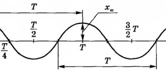
The amplitude of oscillations (Latin amplitude - magnitude) is the greatest deviation of an oscillating body from its equilibrium position.
For a pendulum, this is the maximum distance that the ball moves away from its equilibrium position (figure below). For oscillations with small amplitudes, such a distance can be taken as the length of the arc 01 or 02, and the lengths of these segments.
The amplitude of oscillations is measured in units of length - meters, centimeters, etc. On the oscillation graph, the amplitude is defined as the maximum (modulo) ordinate of the sinusoidal curve (see figure below).
Oscillation frequency.
Oscillation frequency is the number of oscillations performed per unit of time, for example, 1 s.
The SI unit of frequency is named hertz (Hz) in honor of the German physicist G. Hertz (1857-1894). If the oscillation frequency (v) is 1 Hz, this means that one oscillation occurs every second. The frequency and period of oscillations are related by the relations:
.
cyclic or circular frequency is also used . It is related to the usual frequency v and the oscillation period T by the relations:
.
Cyclic frequency is the number of oscillations completed in 2π seconds.
Special cases of formulas for calculating cyclic frequency
A load on a spring (a spring pendulum is an ideal model) performs harmonic oscillations with a circular frequency equal to:
\[{\omega }_0=\sqrt{\frac{k}{m}}\left(7\right),\]
$k$ is the spring elasticity coefficient; $m$ is the mass of the load on the spring.
Small oscillations of a physical pendulum will be approximately harmonic oscillations with a cyclic frequency equal to:
\[{\omega }_0=\sqrt{\frac{mga}{J}}\left(8\right),\]
where $J$ is the moment of inertia of the pendulum relative to the axis of rotation; $a$ is the distance between the center of mass of the pendulum and the suspension point; $m$ is the mass of the pendulum.
An example of a physical pendulum is a mathematical pendulum. The circular frequency of its oscillations is equal to:
\[{\omega }_0=\sqrt{\frac{g}{l}}\left(9\right),\]
where $l$ is the length of the suspension.
The angular frequency of damped oscillations is found as:
\[\omega =\sqrt{{\omega }^2_0-{\delta }^2}\left(10\right),\]
where $\delta $ is the attenuation coefficient; in the case of damped oscillations, ${\omega }_0$ is called the natural angular frequency of oscillations.
Movement examples
Oscillatory motion is one of the most common in nature. For example, you can imagine the strings of a musical instrument, a swing, or a person's vocal cords.
In physics, oscillations are processes that repeat at regular intervals. Such movements are considered through several models:
- a body suspended on a spring (moving up and down);
- weight on a string;
- electrical circuit and others.
Links and notes[edit]
- ^ a b
Cummings, Karen;
Halliday, David (2007). Understanding Physics
. New Delhi: John Wiley & Sons Inc. Authorized reprint for Wiley - India. pp. 449, 484, 485, 487. ISBN 978-81-265-0882-2.(UP1) - Holzner, Stephen (2006). Physics for Dummies
. Hoboken, NJ: Wiley Publishing Inc., p.201. ISBN 978-0-7645-5433-9. angular frequency. - Lerner, Lawrence S. (1996-01-01). Physics for Scientists and Engineers
. paragraph 145. ISBN 978-0-86720-479-7. - Mohr, J.C.; Phillips, W. D. (2015). "Dimensionless units in SI". Metrology
.
52
(1): 40–47. arXiv: 1409.2794. Bibcode: 2015Metro..52…40M. DOI: 10.1088/0026-1394/52/1/40. S2CID 3328342. - Jump up
↑ Mills, I. M. (2016).
"In units of radians and cycle for plane angle quantities." Metrology
.
53
(3):991–997. Bibcode: 2016Metro..53..991M. DOI: 10.1088/0026-1394/53/3/991. - "SI units need to be reformed to avoid confusion". From the editor. Nature
.
548
(7666):135. August 7, 2011. doi:10.1038/548135b. PMID 28796224. - PR Bunker; I.M. Mills; Per Jensen (2019). "Planck's constant and its units." J Quant Spectrosc Radiat Transfer
.
237
: 106594. doi: 10.1016/j.jqsrt.2019.106594. - PR Bunker; Per Jensen (2020). "Plank's Constant Action A." J Quant Spectrosc Radiat Transfer
.
243
: 106835. doi: 10.1016/j.jqsrt.2020.106835. h {\displaystyle h} - Serway, Raymond A.; Jewett, John W. (2006). Fundamentals of Physics
(4th ed.). Belmont, CA: Brooks/Cole - Thomson Learning. pp. 375, 376, 385, 397. ISBN 978-0-534-46479-0. - Nahvi, Mahmoud; Edminister, Joseph (2003). Essay on the theory and problems of electrical circuits by Schaum
. McGraw-Hill Professional. pp. 214, 216. ISBN 0-07-139307-2.(LC1)
Related reading:
- Olenick, Richard P.; Apostle, Tom M.; Goodstein, David L. (2007). Mechanical Universe
. New York: Cambridge University Press. pp. 383–385, 391–395. ISBN 978-0-521-71592-8.
Amplitude, period and frequency
If you simultaneously hang two weights on two different threads and launch them, you will notice that the distance of deviation of the load from the middle position to the extreme position is different.
This quantity is called amplitude. It is designated by the letter A and is measured in the C system in meters. also used to denote such a movement :
- The time it takes for the pendulum to reach the same position is called the period of oscillation.
- The number of oscillations per unit time is frequency. It is measured in Hertz (Hz). It has an inverse relationship with the period.
- The cyclic frequency of oscillations (angular, circular) is the number of oscillations in 2 π seconds. Denoted by the Greek letter omega. It is introduced to simplify calculations in theoretical physics and electronics. The unit of cyclic frequency is rad/s.
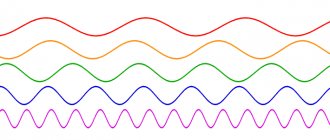
- If there are two graphs of functions with the same frequency, but shifted relative to each other, then their oscillation phase is different.
units
The SI unit of measurement is the hertz. This unit was originally introduced in 1930 by the International Electrotechnical Commission [13], and in 1960 it was adopted for general use by the XI General Conference on Weights and Measures as an SI unit. Previously, the frequency unit was one cycle per second.
(1 cycle per second = 1 Hz) and derivatives as kilocycle per second, megacycle per second, kilometer per second, equal to kilohertz, megahertz and gigahertz respectively).
Math pendulum
This model considers the movement of a load suspended on a thread. A system is described in which the mass of the thread is much less than the mass of the load, and its length is much greater than its dimensions.
Also, the thread should be weightless and inextensible.
The load in this case is considered a material point.
If these conditions are met, the pendulum's oscillation frequency and period will not depend on the mass of the load. The movement of a mathematical pendulum is considered at a small angle of deflection (α). The latter is measured in radians, and therefore approximately corresponds in value to its sine and tangent. The same angle is proportional to the ratio of the displacement to the length of the thread:
α=x/l.
The pendulum is acted upon by the sine component of gravity and the tangent force of tension in the thread. According to Newton's second law: ma=-mgsin (α). Where can I get a=-gx/l
The second derivative of the equation of motion gives a=-(ω)^2x
Thus: -gx/l=-(ω)^2x -> ω ^2=g/l.
Period: T=2π /ω T=2π*sqrt (g/l)
This is Galileo's formula, which describes the movement of a mathematical pendulum.
Formula for oscillation frequency for a mathematical pendulum: v=sqrt (l/g)/2π .
Other Frequency Related Meanings
- Bandwidth
- ν max − ν min {\displaystyle \nu _{max}-\nu _{min}} - Frequency range
- log ( ν max / ν min ) {\displaystyle log(\nu _{max}/\nu _{min})} - Frequency deviation
- Δ ν / 2 {\displaystyle \Delta \nu /2} - Period
- 1 / ν {\displaystyle 1/\nu } - Wavelength
- v / ν {\displaystyle {v}/\nu } - Angular
velocity (rotation speed) - d ϕ / dt ; 2 π FBP. {\displaystyle d\phi /dt;2\pi F_{BP.}}
Spring pendulum
A similar term refers to a system in which movement is performed by a load suspended on a light spring.
The body is in equilibrium if the spring is not deformed. If it is stretched or compressed, the system will begin to oscillate under the action of an elastic force, which is aimed at bringing the pendulum to an equilibrium position.
The elastic force is proportional to the displacement of the body (x), but is directed in the opposite direction. The proportionality coefficient between these two quantities is called the spring stiffness (k). Thus:
F=-kx.
The elastic force reaches its greatest value in the position of maximum deviation of the body (amplitude, displacement) from equilibrium. At this point the acceleration is greatest.
As the body approaches the equilibrium position, the elastic force and acceleration decrease. At the midpoint, both quantities are equal to zero , but the speed of the body has a non-zero value. Therefore, the load does not stop, but continues to move.
After passing the equilibrium position, it moves in the opposite direction by inertia, and the elastic force pulls it back. Due to air friction, the speed decreases and the pendulum stops.
All these models can be classified as a classical harmonic oscillator - a system that has one degree of freedom and is described by a single equation.
Angular velocity
When a body moves in a circle, not all its points move at the same speed relative to the axis of rotation. If we take the blades of an ordinary household fan that rotate around a shaft, then the point located closer to the shaft has a rotation speed greater than the marked point on the edge of the blade. This means they have different linear rotation speeds. At the same time, the angular velocity of all points is the same.
Angular velocity is the change in angle per unit time, not distance. It is denoted by the letter of the Greek alphabet – ω and has a unit of measure: radians per second (rad/s). In other words, angular velocity is a vector tied to the axis of rotation of the object.
The formula for calculating the relationship between rotation angle and time interval is:
Where:
- ω – angular velocity (rad/s);
- ∆ϕ – change in the angle of deflection when turning (rad.);
- ∆t – time spent on deviation (s).
The designation of angular velocity is used when studying the laws of rotation. It is used to describe the motion of all rotating bodies.
Angular velocity in specific cases
In practice, they rarely work with angular velocity values. It is needed in the design development of rotating mechanisms: gearboxes, gearboxes, etc.
You can calculate it using the formula. To do this, use the connection between angular velocity and rotational speed.
Where:
- π – number equal to 3.14;
- ν – rotation speed, (rpm).
As an example, the angular velocity and rotational speed of the wheel disk when moving a walk-behind tractor can be considered. It is often necessary to reduce or increase the speed of the mechanism. To do this, a device in the form of a gearbox is used, with the help of which the speed of rotation of the wheels is reduced. At a maximum speed of 10 km/h, the wheel makes about 60 rpm. After converting minutes to seconds, this value is 1 rpm. After substituting the data into the formula, the result will be:
ω = 2*π*ν = 2*3.14*1 = 6.28 rad/s.
For your information. A reduction in angular velocity is often required in order to increase the torque or tractive effort of mechanisms.
How to determine angular velocity
The principle of determining angular velocity depends on how the circular motion occurs. If uniform, then the formula is used:
If not, then you will have to calculate the values of the instantaneous or average angular velocity.
The quantity we are talking about is a vector quantity, and Maxwell’s rule is used to determine its direction. In common parlance - the gimlet rule. The velocity vector has the same direction as the translational movement of a screw with a right-hand thread.
Oscillatory circuit
Is another example of the oscillation on which all radios are based. The circuit plays the role of a signal receiver.
In the simplest example, it is a closed circuit of an inductor and a capacitor. Under certain circumstances, electrical oscillations can occur and be maintained in such a circuit.
To excite oscillations, it is necessary to connect a constant voltage source to the capacitor and charge it. After this, remove the source and close the circuit.
The capacitor is discharged through the inductor, and a current is created in the circuit, the intensity of which increases as the capacitor is discharged. A magnetic field is created around the coil.
The electrical charge of the capacitor was converted into a magnetic field. After this, the magnetic field of the coil will decrease, and the capacitor will be charged back. The process is repeated cyclically and is described by the same characteristics as mechanical vibrations: frequency, amplitude and period.
They are free and damping. To maintain them, it is necessary to periodically charge the capacitor .
Metrological aspects
To measure frequency, various types of frequency meters are used, including: to measure the frequency of pulses - electron and capacitor counters, to determine the frequencies of spectral components - resonant and heterodyne frequency meters, as well as spectrum analyzers. To reproduce the frequency with a certain accuracy, various measures are used, such as high precision frequency standards, frequency synthesizers, oscillators and others. Frequencies are compared using a frequency comparator or an oscilloscope using Lissajous curves.
Frequency calculation
The frequency of a recurring event is calculated by taking into account the number of times that event occurs within a given period of time. The resulting amount is divided by the duration of the corresponding time interval. For example, if 71 homogeneous events occurred in 15 seconds, then the frequency will be equal to:
ν = 71 15 s ≈ 4 , 7 Hz {\displaystyle \nu ={\frac {71}{15\,{\mbox{s}}}}\approx 4{,}7\,{\mbox{Hz} }}
If the number of samples obtained is small, then a more accurate method is to measure the time interval for a given number of occurrences of the event in question, rather than finding the number of events within a given time interval. [8]. Using this latter method introduces random error between zero and the first sample, averaging half the sample; this can lead to an average error in the calculated frequency Δν = 1/( 2Tm
)
or a relative error Δν /
ν =
1/(
2vTm )
, where
Tm is the time
interval and ν is the measured frequency. The error decreases with increasing frequency; Therefore, this problem is more significant at low frequencies, where the number of samples N is small.
Measurement methods
Stroboscopic method
The use of a special device, a strobe, is one of the historically oldest methods of measuring the rotational speed or vibration of various objects. The measurement uses a strobe light source (usually a bright lamp that periodically produces short flashes of light), the frequency of which is controlled by a pre-calibrated timing circuit. A light source is directed at a rotating object, after which the frequency of flashes gradually changes. When the frequency of flashes is equal to the frequency of rotation or vibration of the object, the latter has time to complete a full cycle of oscillations and return to its original position in the interval between two flashes, so that when illuminated by a strobe lamp, this object will appear motionless. However, this method has a drawback: If the object's rotation frequency (x) is not equal to the strobe frequency (y), but is proportional to it by an integer factor (2x, 3x, etc.), the object will still appear stationary.
The strobe method is also used to adjust the rotation speed (vibration). In this case, the frequency of the flashes is fixed, and the frequency of the periodic movement of the object changes until it begins to appear motionless.
Shaking method
Close to the stroboscopic method is the impact method. It is based on the fact that when mixing oscillations of two frequencies (reference ν
and measuring
ν ' 1 ) in a nonlinear circuit, the frequency difference Δν = |
ν
-
ν' 1 |, called the beat frequency, with linear addition of oscillations this frequency is the frequency of the envelope of the complete oscillation.
The method is applicable when it is preferable to measure low-frequency oscillations with a frequency Δ f
. In radio engineering, this method is also known as the heterodyne frequency measurement method. In particular, the rhythm method is used to tune musical instruments. In this case, sound vibrations of a fixed frequency (for example, from a tuning fork), heard simultaneously with the sound of the instrument being tuned, create a periodic intensification and attenuation of the overall sound. When fine-tuning the device, the frequency of these times tends to zero.
Frequency counter application
High frequencies are usually measured with a frequency meter. It is an electronic device that estimates the frequency of a specific repeating signal and displays the result on a digital display or analogue sensor. The discrete logic elements of a digital frequency meter allow you to take into account the number of periods of signal oscillations within a certain time interval, counted by a reference quartz clock. Periodic processes that are not electrical in nature (such as shaft rotation, mechanical vibration or sound waves) can be converted into a periodic electrical signal using a transducer and thus fed to the input of a frequency meter. Currently, devices of this type are capable of covering a range of up to 100 GHz; this figure represents the practical limit for direct counting methods. The highest frequencies are measured by indirect methods.
Indirect measurement methods
Outside the range accessible to frequency meters, frequencies of electromagnetic signals are often estimated indirectly using local oscillators (i.e., frequency converters). A reference signal of known frequency is combined in a nonlinear mixer (such as a diode) with the signal to be tuned to the frequency; As a result, a heterodyne signal is formed or, alternatively, beats are generated by the frequency difference between the two original signals. If the latter are sufficiently close to each other in their frequency characteristics, then the heterodyne signal is small enough that it can be measured with the same frequency counter. Therefore, this process only estimates the difference between the unknown frequency and the reference frequency, which must be determined by other methods. Multiple mixing stages can be used to cover even higher frequencies. Research is currently underway to extend this method to visible and infrared light frequencies, so-called heterodyne optical detection.