Anti-aliasing filters for power supply rectifiers.
Capacitive, inductive-capacitive, active smoothing filters. Schemes, properties, online calculator.
Kp pulsation coefficient parameter within 10-5 ... 10-4 remained in the air - the nominal value of the smoothing capacitance turns out to be very considerable capacitor.
The ripple factor of the rectified voltage Kp is the most important parameter of the rectifier. Its numerical value is equal to the ratio of the amplitude value of the pulsating voltage to its constant component. Let me remind you of the excerpt from the printed publication given on the previous page:
“The ripple coefficient is chosen independently depending on the expected load, which allows DC power supply of a very certain “purity”: 10-3 ... 10-2 (0.1-1%) - small-sized transistor radios and tape recorders, 10-4 ... 10-3 (0.01-0.1%) - radio and intermediate frequency amplifiers, 10-5... 10-4 (0.001-0.01%) - preliminary stages of audio frequency amplifiers and microphone amplifiers.”
In addition, the concept of filtering coefficient (smoothing coefficient) can be used in the characteristics of rectifiers. The filtering coefficient, also known as the smoothing coefficient , is a value numerically equal to the ratio of the ripple coefficient at the filter input to the ripple coefficient at the filter output Kc = Kp-in/Kp-out . For multi-link filters, the filtration coefficient is equal to the product of the filtration coefficients of individual links.
In low-current circuits, the issue of reducing ripple is solved easily and radically - by using integral stabilizers. The ripple suppression parameter (Ripple Rejection) for such mass-produced ICs is at least 50 dB (360 times the voltage), which, with a high “purity” of the output voltage, makes it possible to reduce the capacitance of electrolytes by 5-10 times.
If the developer does not have the opportunity (or desire) to include voltage stabilizers in the device, then inductive-capacitive or active smoothing filters .
Let's start with filters made of inductive elements - chokes and capacitive elements - capacitors. Fig.1
Figure 1a shows a diagram of the simplest capacitive anti-aliasing filter. The principle of operation is the accumulation of electrical energy by the filter capacitor and the subsequent release of this energy to the load.
In order not to be limited to 50 Hz power supplies, but also to be able to calculate pulse power supply filters, I will give universal formulas that take into account the frequency of the input signal F : C1 = In/(3.14 × Un × F × Kp) for half-wave rectifiers and C1 = In/(6.28×Un×F×Kp) - for full-wave. Kp is the ripple coefficient equal to the ratio of the amplitude value of the ripple voltage to its constant component, and F is the frequency of the alternating voltage at the input of the diode rectifier.
Let's move on to inductive-capacitive LC filters. ATTENTION!!! The need for this kind of circuits arises exclusively in cases where it is necessary to obtain a low level of ripple in sufficiently powerful network power supplies, or in high-frequency switching power supplies. This is due to the fact that for the LC filter to operate effectively, the inductive reactance of the XL coil at the suppression frequency tends to be significantly greater than Rн. And this, in turn, leads to the fact that under conditions of low frequencies and low currents (high Rн), the inductance of the inductor turns out to be unreasonably high.
An L-shaped inductive-capacitive LC filter of the 2nd order (Fig. 1b) has significantly better filtering properties compared to a conventional capacitive one. The product LC (H*μF) depends on the required filter smoothing coefficient and is determined by the approximate formula: L1(H)×C1(μF) = 25000/(F2(Hz)×Kp) for half-wave rectifiers and L1×C1 = 12500/( F2×Kp) - for full-wave, where C1(μF)/L1(mH) = 1000/Rn2(Ohm) .
The diagram of a U-shaped LC filter is shown in Fig. 1c. The smoothing effect of a U-shaped LC filter can be simplified as the combined action of the two filters described above, and the smoothing coefficient as the product of the smoothing coefficients of the links: capacitive and L-shaped inductive-capacitive. Chebyshev LC filters have the best filtering properties. Let's write the formula based on the recommendations set out on the page link to the page: C1 = C2; C1(μF)/L1(mH) = 1176/Rn2(Ohm) .
You can reduce the ripple voltage at the output of a single-link U-shaped LC filter by connecting a non-polar capacitor C3 (Fig. 1d) in parallel with inductor L1 (Fig. 1d) , which, together with the inductance of the coil, forms a notch filter. If the capacitance of capacitor C3 is chosen such that the resonant frequency of the circuit L1-C3 is equal to the ripple frequency (F for half-wave rectification or 2F for full-wave rectification), then most of the ripple voltage will be retained by this circuit and only a small amount will go to the load. So: C3 = 1/(39.44×L1×F2) for half-wave rectifiers and C3 = 1/(9.86×L1×F2) for full-wave rectifiers. All other element values are the same as in the previous diagram.
Let's spice up the material covered with an online table.
CALCULATOR FOR CALCULATING ELEMENTS OF THE POWER SUPPLY COLORING FILTER.
Transistor filters , compared to capacitive smoothing filters, have smaller dimensions, weight and a higher ripple smoothing coefficient. They make it possible to reduce the value of the smoothing capacitor by a factor of ten (at the same ripple level), or to reduce the pulsation amplitude by a similar number of times with a constant capacitance value.
Fig.2
Figure 2a shows a diagram of the most common transistor filter.
The high ripple voltage supplied to the transistor's collector is essentially the supply voltage to the emitter follower formed by T1. At the same time, the base circuit is powered through bias resistors and the integrating circuit R1C1, which smoothes out voltage ripple at the base. The larger the time constant T=R1C1, the less voltage ripple at the base, and since the device is an emitter follower, the ripple at the filter output will be as small as at the base. In order to reduce the dependence of the voltage at the filter output on the level of transmitted power, the current through the divider R1R2 is selected 5...10 times greater than the current branching into the base with minimal load resistance. When calculating the ratings of the divider elements, one should proceed from the voltage at the base of the transistor: Ub = Uin - Uin ripple - (2.5...3V) . In this case, the control transistor will operate in the active mode, and the voltage drop across it will be: Uke = Uin ripple + (3.1...3.6V) . The lower the DC voltage drop across the power transistor, the greater the efficiency of the transistor filter. It is clear from the formula that to ensure high efficiency of an active smoothing filter, a voltage already filtered to a certain level should be supplied to the input of the device . In practice, this is done by connecting a simple capacitive filter to the input (Fig. 1a), the ripple level of which can be calculated using the calculator above.
The effectiveness of active anti-aliasing filters directly depends on the gain of the transistor. The higher the h21 of the semiconductor, the larger the values of the resistors R1, R2 can be chosen - the better filtering properties the circuit will have. Therefore, in this situation you should not even consider transistors with h21
To further improve the filtering properties of the anti-aliasing filter, you can use a two-link RC filter in the base circuit of the transistor (Fig. 2b) . Here, the sum of the resistance values of resistors R1 and R2 is equal to the resistance of resistor R1 in the previous device, and the resistance of resistor R3 is equal to the resistance of resistor R2 in the filter (Fig. 2a).
A transistor filter will work even more efficiently if a zener diode with a breakdown voltage equal to the value calculated for the resistive divider is connected to the base circuit of the transistor instead of R2 (Fig. 1a) or R3 (Fig. 1b).
Rectifiers: Single phase half wave rectifier
The simplest rectifier is the circuit of a single-phase half-wave rectifier (Fig. 3.4-1a). Graphs explaining its operation at a sinusoidal input voltage \(U_{in} = U_{in max} \sin{\left( \omega t \right)}\) are presented in Fig. 3.4-1b.Rice. 3.4-1. Single-phase half-wave rectifier (a) and timing diagrams explaining its operation (b)
Over the time interval \(\left[ {0;} T/2 \right]\), the semiconductor diode of the rectifier is biased in the forward direction and the voltage, and therefore the current in the load resistor repeats the shape of the input signal. In the interval \(\left[ T/2 {;} T \right]\) the diode is reverse biased and the voltage (current) across the load is zero. Thus, the average voltage across the load resistor will be equal to:
\(U_{n avg} = \cfrac{1}{T} {\huge \int \normalsize}_{0}^{T} U_n \operatorname{d}t = \cfrac{1}{T} {\ huge \int \normalsize}_{0}^{T/2} U_{in max} \sin{\left( \omega t \right)} \operatorname{d}t = \)
\(= — \cfrac{U_{in max}}{T \omega} \cos{\left( \omega t \right)}{\huge \vert \normalsize}_{0}^{T/2} \ approx \cfrac{U_{in max}}{\pi} = \sqrt{2} \cfrac{U_{in d}}{\pi}\),
where \(U_{input}\) is the effective value of the alternating voltage at the rectifier input.
Similarly, for average load current:
\(I_{n avg} = \cfrac{1}{2 \pi} {\huge \int \normalsize}_{0}^{\pi} I_{max} \sin{\left( \omega t \right )} \operatorname{d} t \approx \cfrac{I_{max}}{\pi} = {0.318} \cdot I_{max} \),
where \(I_{max}\) is the maximum amplitude of the rectified current.
Effective value of the load current \(I_{n d}\) (the same current flows through the diode):
\(I_{n d} = \sqrt{\cfrac{I_{max}^2}{2 \pi} {\huge \int \normalsize}_{0}^{\pi^{ }} \sin{\ left( \omega t \right)}^2 \operatorname{d} t} = \cfrac{I_{max}}{2} = {0.5} \cdot I_{max} \)
The ratio of the average value of the rectified voltage \(U_{n av}\) to the effective value of the input alternating voltage \(U_{in d}\) is called the rectification coefficient (\(K_{rep}\)). For the scheme under consideration \(K_{out} = {0.45}\).
The maximum reverse voltage on the diode \(U_{rev max} = U_{in max} = \pi U_{n av}\), i.e. more than three times the average rectified voltage (this should be taken into account when choosing a diode for the rectifier).
The spectral composition of the rectified voltage has the form (Fourier series expansion):
\(U_н = \cfrac{1}{\pi} U_{in max} + \cfrac{1}{2} U_{in max} \sin{\left( \omega t \right)} — \cfrac{2 }{3 \pi} \cos{\left( 2 \omega t \right)} — \)
\( — \cfrac{2}{15 \pi} U_{in max} \cos{\left( 4 \omega t \right)} — {…} \)
The ripple factor, equal to the ratio of the amplitude of the lowest (fundamental) ripple harmonic to the average value of the rectified voltage, for the described half-wave rectifier circuit is equal to:
\(K_p = \cfrac{U_{pulse max 01}}{U_{n avg}} = \cfrac{\pi}{2} = {1.57}\).
As can be seen, half-wave rectification has low efficiency due to the high ripple of the rectified voltage.
Another negative aspect of half-wave rectification is associated with the inefficient use of the power transformer from which the alternating voltage is taken. This is due to the fact that in the current of the secondary winding of the transformer there is a constant component equal to the average value of the rectified current. This component is not transformed, i.e.:
\(I_1 \cdot w_1 = \left( I_2 – I_{n av} \right) w_2\) ,
where \(I_1\), \(I_2\) are the currents of the primary and secondary windings, and \(w_1\), \(w_2\) are the number of turns of the primary and secondary windings of the transformer.
The time diagram of the current of the primary winding of the transformer (Fig. 3.4-2) is similar to the current diagram of the secondary winding, but is shifted by the amount \(I_{n av} \cfrac{w_2}{w_1}\).
Rice. 3.4-2. Timing diagram of currents in the primary and secondary windings of a power transformer loaded onto a single-phase half-wave rectifier circuit
In the transformer core, due to the constant component of the secondary winding current, a constant magnetic flux \(\Phi_0 = w_2 \cdot I_0\) is created. This phenomenon is commonly called forced magnetization of the transformer core. It can cause saturation of the transformer magnetic system, i.e. an increase in the no-load current, the effective value of the primary current and, consequently, the calculated power of the primary winding of the transformer, which causes an increase in the required dimensions of the transformer as a whole.
An additional disadvantage of half-wave rectification is the presence of a stable current section, which also reduces the power efficiency of the transformer. The maximum power utilization factor of the transformer for such a circuit does not exceed \(k_{tr P} \approx {0.48}\).
To reduce the level of ripple at the rectifier output, various inductive-capacitive filters are included. The presence of capacitors and inductances in the load circuit has a significant impact on the operation of the rectifier.
In low-power rectifiers, a simple capacitive filter is usually used, which is a capacitor connected in parallel with the load (Fig. 3.4-3).
Rice. 3.4-3. Diagram of a single-phase half-wave rectifier with a capacitive filter (a) and timing diagrams explaining its operation (b)
In steady state operation, when the voltage at the rectifier input \(U_{in}\) is greater than the voltage at the load \(U_n\) and the rectifier diode is open, the capacitor will be recharged, accumulating energy coming from an external source. When the voltage at the rectifier input drops below the opening level of the diode and it closes, the capacitor will begin to discharge through \(R_н\), while preventing a rapid drop in the voltage level across the load. Thus, the resulting voltage at the output of the rectifier (at the load) will no longer be so pulsating, but will be significantly smoothed out, and the more strongly, the larger the capacitance of the capacitor used.
Typically, the capacitance of the filter capacitor is chosen such that its reactance is much less than the load resistance (\(1/ \omega C\ll R_н\)). In this case, the voltage ripple on the load is small and it is acceptable to assume that this voltage is constant (\(U_н \approx {const}\)). Let us accept: \(U_н = U_{in max} \cos{\beta}\), where \(\beta\) is a certain constant that determines the voltage value at the load. Obviously, in the general case, \(\beta\) depends on the capacitor capacity, load resistance, input voltage frequency, etc. The physical meaning of this quantity can be understood from the time diagrams shown in Fig. 3.4-4. As you can see, \(\beta\) reflects the duration of the time interval in one period of external voltage oscillations when the rectifier diode is in the open state (\(\beta = \omega \cdot t_{open}/2\)). The angle \(\beta\) is usually called the cutoff angle.
Rice. 3.4-4. Dependency graph \(A(\beta)\)
For the current flowing through the diode in the open state, we can write:
\( I_d = \cfrac{U_{in} - U_н}{r} \) ,
where \(r\) is the active resistance due to the on-state resistance of the diode and the resistance of the secondary winding of the transformer (sometimes called the rectifier phase resistance).
Considering that \(U_{in} = U_{in max} \sin{\left( \omega t \right)} \):
\(I_d = \cfrac{U_{in max}}{r} \left( \sin{\left( \omega t \right)} - \cos{\left( \beta \right)} \right) = \ cfrac{U_{in max}}{r} \left(\sin{\left(\varphi \right)} — \cos{\left( \beta \right)} \right)\) (3.4.1)
The average value of the rectified diode current over the period (taking into account that the diode is open only in the section \(\varphi = \left[\pi/2 – \beta ; \pi/2 + \beta \right]\):
\(I_{d avg} =\cfrac{1}{2 \pi} {\huge \int \normalsize}_{\frac{\pi}{2} — \beta}^{\frac{\pi}{ 2} + \beta} \cfrac{U_{in max}}{r} \left( \sin{ \left( \varphi \right)} — \cos{\left( \beta \right)} \right) \ operatorname{d} \varphi =\)
\(= \cfrac{U_{in max}}{\pi r} \left( \sin{\left( \beta \right)} — \beta \cos{\left( \beta \right)} \right) \)
Since \(U_{in max} = \cfrac{U_н}{\cos{\left( \beta \right)}} \):
\(I_{d av} =\cfrac{U_н}{\pi r} \cdot \cfrac{\sin{\left( \beta \right)} - \beta \cos{\left( \beta \right)} }{\cos{\left( \beta \right)} } = \cfrac{U_н}{\pi r} A \left( \beta \right) \),
where \( A \left( \beta \right) = \cfrac{\sin{\left( \beta \right)} - \beta \cos{\left( \beta \right)}}{\cos{\left ( \beta \right)}} = \operatorname{tg} \left( \beta \right) — \beta \) (3.4.2)
Formula (3.4.2) is very important when calculating the rectifier. After all, the cutoff angle \(\beta\) is not a pre-known initial parameter; as a rule, it has to be calculated based on the specified output voltage (\(U_н\)), resistance (\(R_н\)) or load current (\(I_н) \)), as well as the parameters of the diode and transformer used (which determine the phase resistance \(r\)). Having these data and taking into account (3.4.2), we can determine the value of the coefficient \(A\):
\(A \left( \beta \right) = \cfrac{I_{d av} \pi r}{U_n} \)
The average current through the diode \(I_{d sr}\) is equal to the average load current \(I_{n sr}\), and given that the voltage across the load is assumed to be constant, then the instantaneous value of the current through the load is equal to the diode current: \( I_n = I_{d av}\). Thus:
\(A \left( \beta \right) = \cfrac{I_{n} \pi r}{U_n} = \cfrac{\pi r}{R_n} \)
To find the cut-off angle \(\beta\) with a known coefficient \(A(\beta)\) in practice, a graph is usually used (Fig. 3.4-4).
The maximum value of the diode current is achieved at \(U_{in} = U_{in max}\) at the time when \(\varphi = \pi/2\), i.e. according to expression (3.4.1):
\( I_{d max} = \cfrac{U_{in max}}{r} \left( 1 — \cos{\left( \beta \right)} \right) = \cfrac{U_n}{r} \ cdot \cfrac{\pi \left( 1 — \cos{\left( \beta \right)} \right)}{\cos{\left( \beta \right)}} \)
And further, taking into account (3.4.2) we obtain:
\( I_{d max} = \cfrac{I_{d avg} \cdot \pi}{A \left( \beta \right)} \cdot \cfrac{1- \cos{\left( \beta \right) }}{\cos{\left( \beta \right)}}\), where \(F \left( \beta \right) = \cfrac{\pi \cdot \left( 1 — \cos{\left( \beta \right)} \right)}{\sin{\left( \beta \right)} — \beta \cos{\left( \beta \right)}}\)
The graph of the function \(F(\beta)\) is shown in Fig. 3.4-5. It shows that as the cutoff angle \(\beta\) decreases, the amplitude of the current through the valves increases significantly.
Rice. 3.4-5. Graph of dependence \(F(\beta)\)
Thus, the capacitive nature of the rectifier load leads to the fact that the rectifier diode is open for a shorter period of time, and the amplitude of the current passing through the diode at this time is greater than in a similar circuit operating on a purely active load. This fact must be taken into account when choosing a diode, which must withstand a repeated current of the appropriate amplitude and, moreover, normally tolerate the initial surge of current when turned on, when the capacitor is initially charged.
This pattern is valid not only for the described single-phase half-wave rectification circuit. The operation of other circuits considered below that have a capacitive load will proceed in a similar way.
The required ripple coefficient at the output of a single-phase half-wave rectifier with a capacitive filter \(K_п\) can be obtained by correctly choosing the capacitance of the smoothing capacitor. To find it, use the following formula:
\( C = \cfrac{H(\beta)}{r \cdot K_п}\),
where \(H(\beta)\) is another auxiliary coefficient, the value of which is found according to the graph (Fig. 3.4-6).
Rice. 3.4-6. Graph of dependence \(H(\beta)\)
A capacitive filter is typical for rectifiers designed for low load currents. For high currents, inductive filters are usually used. Such a filter is an inductor (usually with a ferromagnetic core) connected in series with the load (Fig. 3.4-7). The presence of inductance in the load circuit, as well as capacitance, has a significant impact on the operating mode of the rectifier valves.
Rice. 3.4-7. Diagram of a single-phase half-wave rectifier with an inductive filter (a) and timing diagrams explaining its operation (b)
Operation of the circuit in Fig. 3.4-7 is described by the equation:
\( U_{in max} \sin{\left( \omega t \right)} = L \cfrac{\operatorname{d} I_н}{\operatorname{d} t} + I_н R_н \)
Taking the current in the circuit at the initial moment of time \((t = 0)\) equal to zero, solving this equation we obtain the following expression for the current in the load circuit:
\(I_н(t) = \cfrac{U_{in max}}{\sqrt{R_н^2 + {\left( \omega L \right)}^2}} \left( \sin{\left( \omega t — \theta \right)} + e^{- \cfrac{R_н t}{L}} \sin{( \theta )} \right) \),
where \( \theta = \operatorname{arctg} \left( \cfrac{\omega L}{R_н} \right) \)
A time diagram reflecting this dependence is shown in Fig. 3.4-7(b). It clearly shows the physical meaning of the constant \(\theta\). It represents the angle by which the main current surge in the load lags relative to the voltage surge that initiates it at the rectifier input.
If you analyze the dependence of the load current \(I_н(t)\), you will notice that its amplitude decreases with increasing coil inductance (correspondingly, its average value also decreases). Those. the average voltage across the load turns out to be less than in the case of no inductance, and the output voltage ripple also decreases. The current fluctuations themselves turn out to be shifted relative to the input voltage fluctuations by an angle \(\theta\). This is the reason for the abrupt application of a negative reverse voltage of up to \(U_{rev} = U_{in max}\) to the diode at the moment it is turned off.
The described mode of operation of the valves (drawing current, reducing its amplitude, abrupt application of reverse voltage) in the presence of an inductive filter is typical for all rectifier circuits. An inductive filter is usually used in high-power rectifier circuits, since in this case the inductance required to significantly change the output voltage parameters is insignificant.
The most effective smoothing of rectified voltage ripples is carried out using complex multi-link filters, which include inductors and capacitors (the basis of such filters are the so-called L- or U-shaped links).
| Next > |
Rectified voltage ripple
The considered rectifier circuits made it possible to obtain a rectified but pulsating voltage at the load. Unacceptably large voltage ripples disrupt the normal operation of electronic equipment, create a background at its output, cause signal distortion, and lead to instability of the electronic device as a whole. Therefore, to eliminate rectified voltage ripple
Anti-aliasing filters are included in the rectifier circuit at its output.
| Before getting acquainted with practical filtering circuits, let's consider the physical processes in the circuit of a full-wave rectifier for the case when inductor L is connected in series with the load resistance (Fig. 117, a), i.e., when the rectifier is loaded with inductive and active resistance. The voltage URnL applied to the circuit Rn - L has the form of positive sinusoidal half-waves; the shape of the current flowing through the load differs from the shape of the rectified voltage. As the voltage URnL increases, an e-wave appears in the inductance L. d.s. self-induction eL, which counteracts the increase in current. It is directed towards the increasing voltage URnL and therefore is shown in the graph with reverse polarity. Rice. 117. Operation of a full-wave rectifier: a - for inductance and active resistance; b - for capacitance and active resistance. |
As soon as the current of the first valve B1 stops increasing (reaches a maximum), e. d.s. self-induction becomes zero. In the next part of the period, when its polarity changes, it will prevent the current in the circuit Rн - L from decreasing, so the current stops not at the moment, but later, at time t'. At time t', valve B2 also opens and the current in the load is the sum of the increasing current of valve B2 and the decreasing current of valve B1, supported by e. d.s. self-induction (the latter now closes through valve B2, since valve B1 is locked).
The average value of the rectified current is already slightly different from the maximum current through the valve, and this difference will be smaller, the greater the inductance L. At the same time, the ripple of the rectified voltage
. So, at ωL, - (5÷8) Rн, voltage ripples at the load do not exceed 20%.
The reverse voltage on the valve is equal to the sum of e. d.s. eII and voltage at the input of the Rн-L circuit:
Uob.max2EmII≈πUsr.
In general, the average value of the rectified voltage across the load is
Usr = Usr.x.x - Isr (Ri + rII + rdr),
where Uav.х.х is the voltage at the rectifier output when the load is off in idle mode; Iav (Ri + rII + rdr) - loss voltage at the active resistances of the circuit elements.
From the last equality it follows that with an increase in the current through the load (with a decrease in Rн), the slope of the external characteristic increases. However, this slope does not depend on the inductance of the inductor, therefore, in a rectifier with an inductive load, it is advisable to use valves with low internal resistance Ri (selenium or ion valves).
In Fig. 117, b shows a full-wave rectifier circuit loaded on a parallel-connected capacitor C and resistance Rн, as well as graphs explaining the operation of this circuit.
The capacitor is recharged twice each period to voltage UC.max alternately through valve B1 and valve B2. When the voltage on the corresponding half of the secondary winding of the transformer becomes higher than the voltage UC on the capacitor, it. it is recharged in the time intervals t1 - t2, t3 - t4 and discharged to the load in the time intervals t2 - t3, t4 - t5. In this case, the current in the load is maintained due to the energy accumulated in the capacitor. The valves are locked at this time. The greater the load resistance, the slower the capacitor discharges, the less the voltage across the load changes (pulsates less).
The average value of the rectified voltage is approximately equal to the voltage amplitude on half of the secondary winding of the transformer: the reverse voltage is 2 times higher (≈2EmII), the ripple coefficient does not exceed 15% at C≈8÷10 µF.
It should be noted that the current in the load flows throughout the entire half-cycle, while the current through the valve passes only part of the half-cycle, and the maximum value of this current is 3-4 times greater than the average rectified value. Therefore, if it is necessary to obtain a current of 100 mA from the rectifier, then the permissible maximum valve current must be at least 300 mA.
The slope of the external characteristic depends not only on the value of the internal resistance of the valve and the secondary winding of the transformer, but also on the time constants for charging and discharging the capacitor:
tzar ≈ С(Ri+r'II); trazr = CRn
The magnitude of the rectified voltage depends sharply on the magnitude of the load current. When Rн = ∞, i.e., when Iср = 0, the voltage across the capacitance is maximum; as Rн decreases, the voltage Uср drops.
A rectifier operating on capacitance can be considered as a source with high internal resistance. At the moment the circuit is turned on, an inrush of current occurs, the initial charge of capacitor C occurs, the current in the circuit is limited only by the internal resistance of the valves, so there is a danger of one of them failing.
Ripple factor
| [Home] | [Donate!] [Contacts] |
Ripple factor
Ripple coefficient is the ratio of the absolute level of ripple to the constant component of the signal. In other words, the pulsation coefficient is a measure of pulsation in relative units. Despite the fact that it would seem that this concept can be given a fairly clear definition, in fact it is extremely ambiguous. The reason for this is that there are completely different approaches to determining the absolute level of ripple.
Contents Pulsation coefficient Introduction Definition of pulsation coefficient Definitions of the concept in accordance with regulatory documentation Alternative definitions Sources of information
Introduction
Quite often, for example, when measuring various physical quantities, when analyzing the quality of the power supply of devices and when considering many other issues, we are faced with the phenomenon of ripple - an undesirable periodic deviation of a value (for example, the output voltage of a power supply) relative to the average value.
The measure of pulsation is the level of pulsation, which can be expressed in absolute values (ripple amplitude, peak-to-peak, effective value, etc.). But sometimes it is convenient to consider the pulsation level not in absolute terms, but in relative units. The ratio of the quantity characterizing the level of ripple to the constant component of the signal is called ripple coefficient .
The ripple factor can be used, for example, as an objective characteristic of the quality of the output voltage of a power supply, which allows you to compare different devices with each other, without reference to the absolute values of the output voltages. The ripple coefficient makes it possible to judge the applicability of a given source for powering a particular load, because to ensure the operability of the consumer, the ripple should not exceed the permissible limits specified for it.
Another simple example where considering ripple factor is useful is in the analysis of rectifiers. Thus, for an idealized rectifier without a smoothing filter, the ripple factor is a circuit parameter that does not depend on either the input voltage or the load and makes it possible to easily compare different types of rectifiers.
Determination of ripple factor
Some difficulties with using this parameter arise due to the fact that many different pulsation coefficients can be introduced into consideration, depending on what value we choose as an absolute measure of the pulsation level. Therefore, it is important to clarify exactly what coefficient we are talking about. This is something that some authors sometimes neglect, and then one can only guess what was meant.
There are three main approaches to determining the pulsation coefficient, which are most often used in the literature and are reflected in regulatory documentation (standards).
1. Pulsation coefficient - the ratio of half the pulsation peak-to-peak to the average value of a quantity (or, which is the same thing, to the constant component of the quantity). The ripple range is understood as the difference between the maximum and minimum value: $$ k=\frac {U_{max}-U_{min}} {2 U_0}. $$
Rice. %img:rpl_def
For practical measurement of the ripple coefficient, it is convenient to use an oscilloscope and determine the values of Umin, Umax. If we use the approximation \(U_0 \approx (U_{min}+U_{max})/2,\) to estimate the constant component, we obtain the following formula, convenient for the practical determination of the pulsation coefficient: $$ k \approx \frac {U_{ max}-U_{min}} {U_{max}+U_{min}}. $$
There is a similar definition, but it uses not half the swing, but the full swing of the pulsations.
2. Pulsation coefficient - the ratio of the ripple amplitude to the average value of the quantity (to the constant component of the quantity): $$ k=\frac {U_{max}-U_{min}} {U_0}, $$ or, in a more convenient form for calculation based on the measurement results we will write it as $$ k \approx 2 \; \frac {U_{max}-U_{min}} {U_{max}+U_{min}}. $$
But you can use not only the amplitude values of the ripple value, but, for example, the effective (rms) value of the ripple voltage. Then we get the following definition.
3. Ripple coefficient - the ratio of the root-mean-square value of the variable component to the absolute value of the constant component of the changing quantity: $$ k=\frac {U_{eff}} {U_0}. $$
Each of the considered definitions has its own scope. The choice is determined by which coefficient best reflects the actual pulsation characteristics in a given case.
The coefficients calculated from the amplitude and amplitude of the pulsation (the first and second definitions) are generally equivalent, they only differ from each other by a factor of 2. They characterize the greatest deviation of a value from the average value. Well suited, for example, for assessing the quality of the output voltage of power supplies. As a rule, the powered device has very specific requirements for peak deviations of the supply voltage, which allows, based on the amplitude ripple coefficient, to draw a conclusion about the applicability of the ripple source.
In some cases, it is not the amplitude that is of greater interest, but the effective value of the ripple, which determines the ripple power on a resistive load. And then they give preference to the third definition.
The effective value of the quantity, and therefore the pulsation coefficient calculated from it, turns out to be insensitive to single short-term spikes in the quantity (“needles” of the signal), which correspond to low energy transferred to the load and which make a small contribution to the average power dissipated by the load.
Sometimes this feature of the RMS ripple factor turns out to be useful.
Definitions of the concept in accordance with regulatory documentation
Since the ripple factor is a very important technical parameter, it is not ignored in the standards.
Let's see, for example, what can be found on this issue in the standards of the fairly authoritative organization IEC (International Electrotechnical Commission). As part of its standards development activities, the IEC has also done a great deal of work to unify terminology in the field of electrical engineering, resulting in the creation of the International Electrotechnical Dictionary (Electropedia), which is available online.
Using a dictionary search, we find that the terms “pulsation” and “pulsation coefficient” are used in different subject areas: mathematics; electromagnetic compatibility; power electronics, etc. This is another reason for the ambiguity of the term.
If, for example, we turn to the section on electromagnetic compatibility, we will find that two types of ripple coefficients are considered there:
- peak-ripple factor (ripple factor by amplitude value, peak ripple factor) - the ratio of the peak value of the variable component to the absolute value of the constant component of the changing quantity (translation of the definition from document IEC-60050-161; the peak value simply means the peak-to-peak ripple)*;
- rms-ripple factor (rms ripple factor, root mean square ripple factor) - the ratio of the rms value of the variable component to the absolute value of the constant component of the changing quantity (translation of the definition from document IEC-60050-161; rms value is what used to be called actual value).
* English version: peak-ripple factor — the ratio of the peak-to-valley value of the ripple content to the absolute value of the direct component of a pulsating quantity. The meaning of the term "peak-to-valley value" can also be found in Electropedia: peak-to-valley value, peak-to-peak value - difference between the global maximum value and the global minimum value in the same specified interval of the argument . Note 1 to entry: For a periodic quantity, the specified interval has a range equal to the period. Note 2 to entry: The synonym “peak-to-peak value” should be used only when the global maximum and minimum values are of different signs.
In the “Power Electronics” section we find the term “DC ripple factor”, which is defined as the ratio of half the difference between the maximum and minimum value of the ripple current to the average value of this current (ratio of half the difference between the maximum and minimum value of a pulsating direct current to the mean value of this current), see IEC-60050-551. This definition is similar to the previously discussed definition for the peak-ripple factor (ripple factor by amplitude value), but here, not the full ripple peak-to-peak is taken for calculation, but half.
There are probably reasons for introducing two similar definitions, but this does not help get rid of the confusion at all.
You can also find a mention of the pulsation coefficient in GOST. Thus, in many articles concerning the topic of pulsation, a reference is made to “GOST 23875-88 Quality of electrical energy. Terms and Definitions”, which provides several definition options:
- Voltage (current) ripple coefficient is a value equal to the ratio of the largest value of the variable component* of the pulsating voltage (current) to its constant component. Note. For standardization purposes, it is allowed to refer to the rated voltage (current). * It is not entirely obvious what is meant by “the largest value of the variable component.” Perhaps it's the amplitude.
- The voltage (current) ripple coefficient based on the effective value is a value equal to the ratio of the effective value of the alternating component of the pulsating voltage (current) to its direct component.
- The average voltage (current) ripple coefficient is a value equal to the ratio of the average value of the variable component of the pulsating voltage (current) to its constant component.
The first two definitions have their counterparts in the IEC, but the last one is something new. And again, there was a bit of mystery involved. Since the average value of the variable component is 0, it can be assumed that something else was meant in the definition. Most likely, this is the “modulo-average value of alternating voltage (current),” which in the same GOST is defined as “the period-average modulus value of the instantaneous values of alternating voltage (current).” It probably makes sense to use this coefficient in some cases.
Having considered in such detail the issue of pulsation coefficient from the point of view of GOST 23875-88, it remains only to note that this GOST has become invalid since 2012. So now the reference to it looks like a not very convincing justification for using one definition or another*.
* However, for example, in the current GOST 23414-84 Semiconductor power converters. Terms and definitions (with Amendment No. 1)” contains a reference to the no longer valid GOST 23875-88. It turns out that this is possible.
However, here other GOSTs come to our aid. Thus, in “GOST 26567-85 Semiconductor power converters. Test methods" (at the time of writing this article has a valid status), a visual explanation is given "in pictures", Fig. %img:h. In the figure: 1 - envelope of instantaneous values of pulsating voltage; t is the time during which observations are made. As we can see, half the pulsation amplitude is taken as the pulsation value. The calculation formula is also given (for calculating the coefficient as a percentage): $$ k_{pool}=\frac{U_{pool}}{U_{nom}}\cdot 100, $$ i.e. the ratio of half the ripple peak-to-peak to the nominal value.
Rice. %img:h
This definition is somewhat similar to the “DC ripple factor” definition discussed above from IEC-60050-551.
Similar definitions can be found in other GOSTs, for example, in “GOST R 52907-2008 Power sources for radio-electronic equipment. Terms and definitions: the pulsation coefficient of the direct output voltage [current] of the electronic power supply source is a value equal to the ratio of the largest value of the alternating component of the pulsating direct output voltage [current] to its average value in the steady state of operation of the power supply of electronic equipment.
True, this standard is national (as hinted at by the P symbol in the designation), but still.
Alternative definitions
To be fair, it should be noted that the definitions of the pulsation coefficient discussed above are not the only possible ones and other options can be found in the literature.
In principle, the pulsation coefficient can be understood as the ratio of any measure of the pulsation level to the average value. Therefore, if necessary, the most exotic definition options can be introduced into consideration. For example, we can take the sum of the harmonics of the variable component with weighting coefficients convenient for us as the ripple level.
In the simplest case, we take the first harmonic with a coefficient of 1 and get another version of the definition, which can be found quite often in the domestic literature: the ripple coefficient is the ratio of the amplitude of the first harmonic (or the lowest, or the fundamental - in different formulations) to the average voltage value (i.e. e., to the constant component).
However, a certain degree of popularity does not mean that this definition is successful. Firstly, all harmonic components except the “main” are excluded from consideration, while the contribution of the “non-fundamental” can be very significant; As a result, the resulting coefficient very indirectly reflects the real state of affairs. Secondly, the practical measurement of the coefficient is not simple - it requires isolation (filtering) of one harmonic to measure its amplitude.
But if, for example, we are dealing with the power supply of a device for which very specific components in the pulsation spectrum are standardized, then the described definition option is quite suitable.
Information sources
- IEC, International Electrotechnical Commission.
- Electropedia (International Electrotechnical Dictionary).
- GOST 26567-85 Semiconductor power converters. Test methods
- GOST R 52907-2008 Power supplies for radio-electronic equipment. Terms and Definitions
- GOST 23414-84 Semiconductor power converters. Terms and definitions (with Amendment No. 1)
- GOST 23875-88 Quality of electrical energy. Terms and Definitions
author: hammer; date: 2019-12-01; updated: 2021-10-29
Definition and formula of ripple factor
Voltage ripple coefficient (Kp) is a value that determines the ratio of the maximum component of the alternating voltage (Uac.max.) to its constant component (Uconst). For convenience, it is expressed as a percentage.
Calculation of voltage ripple factor
Current ripples are calculated in the same way.
Calculation of current ripple factor
Iper. Max. is the alternating component of the current. Iconst. is its constant component.