Physical meaning of magnetic induction (MI)
The ability to act on an object with a magnetic field (MF) determines the essence of true induction. It appears at the moment a magnet of a permanent nature moves in the inductance coil. The result of such movement is the appearance of current, with a simultaneous increase in magnetic flux. Since the winding of the coil is metal, and the metal structure is a crystal lattice, the physical properties of this phenomenon can be explained.
The electrons located in this lattice are at rest in the absence of magnetic influence. There is no movement. It begins at the moment when electrons come under the influence of an alternating magnetic field (the field changes when the permanent magnet moves).
The value of the current arising in the coil depends on the diameter of the core and the number of turns, the physical characteristics of the magnet and the speed of its movement.
The unit of dimension in the C system of the characteristic under consideration is tesla. It is designated by the letters Tl.
Important! The electrons in the lattice, after the coil enters the MP, turn at a certain angle and line up along the field lines of the MP. The number of oriented particles and the uniformity of their placement depend on the field strength.
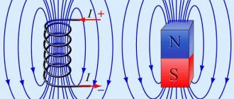
Vector is the magnetic field induction vector (gradient parameter of the magnetic field).
Magnetic induction vector
The phenomenon of electromagnetic induction
Electromagnetic induction is the phenomenon of the occurrence of current in a closed conductive circuit when the magnetic flux passing through it changes.
The phenomenon of electromagnetic induction was discovered by M. Faraday.
Faraday's experiments
- Two coils were wound on one non-conducting base: the turns of the first coil were located between the turns of the second. The turns of one coil were closed to a galvanometer, and the second was connected to a current source. When the key was closed and current flowed through the second coil, a current pulse arose in the first. When the switch was opened, a current pulse was also observed, but the current through the galvanometer flowed in the opposite direction.
- The first coil was connected to a current source, the second, connected to a galvanometer, moved relative to it. As the coil approached or moved away, the current was recorded.
- The coil is closed to the galvanometer, and the magnet moves - moves in (extends) - relative to the coil.
Experiments have shown that induced current occurs only when the magnetic induction lines change. The direction of the current will be different when the number of lines increases and when they decrease.
The strength of the induction current depends on the rate of change of the magnetic flux. The field itself may change, or the circuit may move in a non-uniform magnetic field.
Explanations of the occurrence of induction current
Current in a circuit can exist when external forces act on free charges. The work done by these forces to move a single positive charge along a closed loop is equal to the emf. This means that when the number of magnetic lines through the surface limited by the contour changes, an emf appears in it, which is called the induced emf.
Electrons in a stationary conductor can only be driven by an electric field. This electric field is generated by a time-varying magnetic field. It is called the vortex electric field. The concept of a vortex electric field was introduced into physics by the great English physicist J. Maxwell in 1861.
Properties of the vortex electric field:
- source – alternating magnetic field;
- detected by the effect on the charge;
- is not potential;
- the field lines are closed.
It will be interesting➡ NPN transistor
The work of this field when moving a single positive charge along a closed circuit is equal to the induced emf in a stationary conductor.
MI vector direction
The direction of magnetic fields can be indicated by a magnet arrow placed in these fields. It will spin until it stops. The northern end of the arrow will show where B→ the unit vector of a particular field is oriented.
Magnetic induction lines
The frame with current behaves in the same way, having the ability to navigate the MP without interference. The direction of the induction vector indicates the orientation of the normal to such a closed electromagnetic circuit.
Attention! The rule of the gimlet (right screw) is used here. If the screw is rotated in the direction of the current in the frame, then the forward movement of the screw will coincide with the direction of the positive normal.
In some cases, the right-hand rule is used to find direction.
Direction determination B→
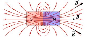
Visual display of MI lines
The line to which a tangent can be drawn, coinciding with B→, is called the magnetic induction (MI) line. Using such lines, you can visually display the magnetic field. These are closed contour lines that cover currents. Their density is always proportional to the value of B→ at a specific point in the MP.
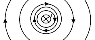
Information. When dealing with the magnetic field of direct motion of charged particles, these lines are depicted as concentric circles. They have their center located in a straight line with the current, and are located in planes located at right angles to it.
The direction of magnetic lines can also be determined using the gimlet rule.
Graphic designation of MI lines
Transformer core material
It is often believed that pulse transformers should be made on ferrites. This is only partly true. Many pulse devices operate at fairly low frequencies. If the frequency is less than 3 kHz, then transformer hardware is definitely a justified choice. At frequencies 3 - 7 kHz the choice is not obvious. For frequencies above 7 kHz, ferrites will be required. Now cores made of powdered iron have appeared. They combine the advantages of ferrite and transformer iron and perform well at frequencies up to 100 kHz. However, they are not yet widely available.
Here is a selection of materials for your attention:
Design of power supplies and voltage converters Development of power supplies and voltage converters. Typical schemes. Examples of finished devices. Online payment. Opportunity for authors
The practice of electronic circuit design. The art of device development. Element base. Typical schemes. Examples of finished devices. Detailed descriptions. Online payment. Opportunity to ask questions to the authors
Magnetic induction vector module
Law of Electromagnetic Induction - Formula
To determine the magnitude of the MI vector, you need to know its module. How is the magnitude of the magnetic induction vector (gradient) determined? This can be understood using a small model as an example. If you place a horizontally suspended conductor in the field of a horseshoe magnet, then the magnetic field of the magnet will act only on the area located in the interpolar gap. The force F→ acting on this section will be directed at right angles to the induction lines and the conductor itself. It reaches its maximum when the ort MI is located perpendicular to the conductor.
The value of the modulus B→ will be equal to the ratio of the maximum value of this force F → to the product of the length of the segment ∆ L by the force of movement of the charges ( I ), namely:
B = Fm/I*∆L.
Electrical model for determining module B→
Units of measurement of magnetic quantities.
The System of Units (SI) defines units of magnetic quantities based on the laws of electromagnetism through corresponding electrical and mechanical units.
Maximum tension
takes place on the outer surface of the conductor. A magnetic field also arises inside the conductor, but its intensity decreases in the direction from the outer surface to its axis. Magnetic field strength H is measured in amperes per meter (A/m).
1 A/m is the magnetic field strength excited by a current of 12.566 A of a straight, infinitely long conductor at a distance of 2 m from its axis. The unit dimension (A/m) and its definition are given based on the law of total current.
Magnetic flux
F is measured in webers (Wb). 1 Wb is equal to such a magnetic flux, when it decreases to zero in 1 s, an induced emf equal to 1 V appears in the circuit linked to this magnetic flux: Wb = V • s.
Magnetic induction B
measured in teslas (T). 1 T is the induction of such a uniform magnetic field in which the magnetic flux through an area of 1 m2 perpendicular to the direction of the magnetic field is equal to one 1Wb: T = Wb/m2.
Absolute magnetic permeability and magnetic constant
measured in . Since, therefore, the unit of absolute magnetic permeability must be measured in
Inductance is measured in henry (H). An inductance of 1 Gn has a circuit in which a current of 1 A creates a magnetic flux of 1 Wb coupled to the circuit. Since Gn = , the unit will be Gn/m.
Along with the SI systems, it is allowed to use magnetic units of the non-rationalized electromagnetic system SGS, the main units of which are centimeter, gram, second. The formulas of electromagnetism in this system are not rationalized; they contain a coefficient.
In this system the tension is H
measured in oersteds (O):
Magnetic flux Ф is measured in maxwells (Mks). 1 Wb = 108 Mks.
Magnetic induction B is measured in gauss (G). 1 T = 104 Gs,
Inductance is measured in centimeters (cm). 1 Gn = 109cm.
Total current law
determines the dependence of the magnetic field strength on the currents that excite it. In the simplest case, the magnetic field strength H of a straight long wire at a distance x from its axis will be:
Here is the length of a circle circumscribed around a wire of radius x.
At all points of this circle, due to the symmetry of the system, the magnetic field strength is the same, and the circle itself coincides with the magnetic line described around the conductor
The structure of the magnetic system and the principle of its calculation
The magnetic flux in an electric motor arises due to the presence of current in the windings: in direct current and synchronous machines, direct current passes through the excitation windings, and alternating current passes through the armature windings; in asynchronous machines and transformers, alternating current passes through all windings.
In (fig.) a part of a four-pole DC machine is shown in schematic form and a picture of the magnetic flux created by the main poles is shown (additional poles are not shown so as not to clutter the drawing). Due to the complete symmetry of the machine, the flux created by each of the poles is divided relative to the longitudinal centerline of the pole into two parts, forming two identical magnetic circuits located symmetrically on both sides of the centerline of a given pole. The number of such circuits is equal to the number of poles of the 2p machine, but when calculating the magnetizing force it is enough to keep in mind only one of them.
To improve the magnetic connection between the windings and increase the magnetic flux, the magnetic system of the machines is made of ferromagnetic materials with good magnetic conductivity. In most cases, electrical steel alloyed with silicon is used (1 -5.0%) and
other additives that reduce losses in an alternating magnetic field.
The main flux Fo is only part of the magnetic field created by the pole. The other part of the magnetic field, called the leakage flux Fa, branches into the space between the poles and, therefore, does not pass into the armature and does not participate in the creation of the emf (Fig. 3).
The purpose of calculating the magnetic system is to establish a connection between the magnetic flux Fo and the currents in the EM windings.
The entire path of the magnetic flux in a DC electric machine consists of five sections (see Fig. 3): an air gap with a length of 25, a tooth layer with a length of 2hz,
armature core length La, pole core length 2hn, frame length £с.
Since the magnetic flux in the cross section of the machine is distributed symmetrically relative to the longitudinal axes of the poles, the calculation of the magnetic circuit is carried out for 1/2p of the machine (see Fig. 3).
According to the law of the magnetic circuit:
(8)
where is the magnetic resistance of the circuit
Here Lk -
the length of the magnetic circuit section, Sk is the cross-sectional area of the magnetic circuit section, µk is the magnetic permeability of the magnetic circuit section.
Hence, the magnetizing force (NS) of the field winding
(9)
where: - magnetizing force along the magnetic circuit;
— magnetic flux of an elementary tube;
— tube length element;
— magnetic permeability of bodies and media forming a given section of the circuit;
— section of an elementary tube.
When calculating the main n. With. Fo machines
we divide the magnetic circuit of the machine into sections in such a way that within each of these sections it can be assumed that the magnetic flux of the tube, its permeability and cross-section remain constant along the entire length of the tube. Under these conditions, we consider the magnetic flux of each section as consisting of a certain number of identical elementary tubes, each having a length l, and uniformly distributed over the cross-sectional area S of this section. The values characteristic for each section of the magnetic circuit are given in Table 1.
It should be taken into account that the length of the elementary tubes (magnetic lines) in the sections in the yoke and in the back of the armature is not the same, therefore the calculation of n. With. These sections are led along the length of the average magnetic line (see figure).
Then the main n. With. a machine designed for a pair of poles can be written as:
(10)
Since, according to the condition, the magnetic flux is distributed evenly over the cross section of each section, then
(11)
Under these conditions, equation (1) is rewritten as follows:
(12)
Equation (12) shows that to determine n. With. XFo needs to find the corresponding magnetic field strength Hg for each of the five sections
and multiply it by the length of the flow path in this section. Since , the magnetic field strength of a given area depends on the magnitude of the magnetic induction and the magnetic permeability of the material of the area. If the magnetic flux and geometric dimensions of all sections are given, then the magnetic induction of the section is determined according to formula (2.12). The magnetic permeability of an area depends on the magnetic properties of the material of this area. For non-magnetic materials, in particular, for the air gap, we have: µ0 = 4π 10-7 H/m in the rationalized MCSA and SI systems; µ0 = 4π in the rationalized GHS system. In practice, when calculating the magnetic circuits of electric machines, a mixed system is used, which is based on the SGSM system with the conversion of units of voltage, current, power, etc. into practical units - volts, amperes, watts, etc. In this case, μ0 = 4π 10-1.
Knowing the induction for a given material, we can determine the magnetic field strength H
and plot the magnetization curve B = f(H) of this material.
Basic formulas for calculating the MI vector
The magnetic induction vector, the formula of which is B = Fm/I*∆L, can be found using other mathematical calculations.
Biot-Savart-Laplace Law
Induction EMF formula
Describes the rules for finding B→ magnetic field, which creates a constant electric current. This is an experimentally established pattern. Biot and Savard identified it in practice in 1820, Laplace managed to formulate it. This law is fundamental in magnetostatics. During the practical experiment, a stationary wire with a small cross-section was considered, through which an electric current was passed. For study, a small section of wire was selected, which was characterized by the vector dl. Its module corresponded to the length of the section under consideration, and its direction coincided with the direction of the current.
Interesting. Laplace Pierre Simon proposed to consider even the movement of one electron as a current and, based on this statement, using this law, he proved the possibility of determining the magnetic field of an advancing point charge.
According to this physical rule, each segment dl of a conductor through which electric current I flows forms dB r and at an angle α :
dB = µ0 *I*dl*sin α /4*π*r2,
Where:
- dB – magnetic induction, T;
- µ0 = 4 π*10-7 – magnetic constant, H/m;
- I – current strength, A;
- dl – conductor section, m;
- r – distance to the point where the magnetic induction is located, m;
- α is the angle formed by r and the vector dl.
Important! According to the Biot-Savart-Laplace law, by summing the magnetic field vectors of individual sectors, it is possible to determine the MF of the desired current. It will be equal to the vector sum.
Biot-Savart-Laplace Law
There are formulas that describe this law for individual cases of MP:
- fields of direct movement of electrons;
- fields of circular motion of charged particles.
The formula for MP of the first type is:
B = µ* µ0*2*I/4*π*r.
For circular motion it looks like this:
B = µ*µ0*I/4*π*r.
In these formulas, µ is the magnetic permeability of the medium (relative).
The law under consideration follows from Maxwell's equations. Maxwell derived two equations for the magnetic field; the case where the electric field is constant is considered by Biot and Savart.
Superposition principle
For MF, there is a principle according to which the total vector of magnetic induction at a certain point is equal to the vector sum of all MI vectors created by different currents at a given point:
B→= B1→+ B2→+ B3→… + Bn→
Superposition principle
Circulation theorem
Initially, in 1826, Andre Ampère formulated this theorem. He analyzed the case with constant electric fields, his theorem is applicable to magnetostatics. The theorem states: the circulation of MF of direct electricity along any circuit is proportional to the sum of the forces of all currents that penetrate this circuit.
Worth knowing! Thirty-five years later, D. Maxwell generalized this statement, drawing parallels with hydrodynamics.
Another name for the theorem is Ampere’s law, which describes the circulation of MP.
Mathematically, the theorem is written as follows.
Mathematical formula of the circulation theorem
Where:
- B→– magnetic induction vector;
- j→ – electron motion density.
This is the integral form of writing the theorem. Here, on the left side one integrates along a certain closed contour, on the right side - along a stretched surface onto the resulting contour.
Magnetic flux
One of the physical quantities characterizing the level of magnetic field crossing any surface is magnetic flux. It is designated by the letter φ and has a unit of measurement called Weber (Wb). This unit is characteristic of the SI system. In the GHS, magnetic flux is measured in maxwells (Mks):
108 μs = 1 Wb.
Magnetic flux φ determines the magnitude of the magnetic field penetrating a certain surface. The flux φ depends on the angle at which the field penetrates the surface and the strength of the field.
The formula for calculation is:
φ = |B*S| = B*S*cosα,
Where:
- B is the scalar value of the magnetic induction gradient;
- S – area of the intersected surface;
- α is the angle formed by the flow Ф and the perpendicular to the surface (normal).
Attention! Flux Ф will be greatest when B→ coincides with the normal in direction (angle α = 00). Similar to Ф = 0, when it runs parallel to the normal (angle α = 900).
Magnetic flux
The magnetic induction vector, or magnetic induction, indicates the direction of the field. Using simple methods: the gimlet rule, a freely oriented magnetic needle or a circuit with a current in a magnetic field, you can determine the direction of action of this field.
Magnetic field: all formulas
Flat circuits—closed conductors made from the finest wire—carrying current are placed in a uniform field. Peak torque measurements show that it:
- directly proportional to the strength of the electric current I flowing through the circuit;
- depends on the contour area S;
- does not depend on the shape of the closed conductor with equal area.
The magnetic moment of the circuit with current is equal to:
pm = IS.
Let's consider the remaining formulas that allow us to calculate the electromagnetic field.
Rotating and magnetic moments characterize electromagnetic induction; in modulus it is equal to:
B= Mmax : pm.
Measured in teslas (T), named after the greatest Serbian scientist of the 20th century, Nikola Tesla.
When calculating inhomogeneous fields, small contours are placed in them, their dimensions comparable to the distances at which changes are observed.
A magnetic field formation is characterized by a strength H proportional to the induction in a vacuum:
B = μ0H,
μ0 = 4π*10-7 H/m or T*m/A.
When calculating for a substance, the magnetic permeability coefficient μ is added; for a vacuum it is equal to unity.
B = μ μ0H.
Magnetic induction of solenoid:
B = μ0nI, here:
- n = N: l, N – number of turns of the coil, l – its length;
- I is the strength of the flowing current.
Formula for magnetic field energy W for a solenoid:
W = LI2: 2 = ФI: 2
- L – coil inductance;
- I – current strength;
- F – magnetic flux.
The force of interaction between conductors with electric current:
F = μ μ0I1I2l : 2πr, here:
- I1, I2 – current strength in both conductors;
- l – their length;
- r – distance between wires carrying current.
Highest moment:
Mmax=BIS;
S – contour area.
An electromagnetic field is formed around magnetized bodies and current-carrying conductors.
Share on social networks: October 18, 2022, 18:15 Physics 0.00% 00