In electrical circuits there is always a magnetic field, which has an electromagnetic interaction with the currents of these circuits. This factor is taken into account when calculating circuits, and the law of total current for the magnetic field is a tool for such calculations.
If you bring a magnetic needle close to a conductor through which current flows, its position will change. This indicates the presence around the conductor, in addition to the electric one, also of a magnetic field. As a result of numerous studies of electromagnetic phenomena, it has been established that there is a mutual influence of fields of electric and magnetic nature.
Physical meaning of the law
Let's consider a simplified version of the influence of magnetic induction on the electric field. To do this, imagine two parallel conductors through which direct currents circulate, for example, I1 and I2. A field is formed near these conductors, which can be mentally limited by a certain contour L - an imaginary closed figure, the plane of which intersects the flows of moving charges.
Within the plane covered by the contour L, a magnetic field is formed, the intensity of which is distributed in accordance with the directions of the currents. In this case, the circulation of the magnetic field vector in the plane of a closed circuit is directly proportional to the sum of the currents piercing this circuit. The total electric current is equal to the vector sum of its components:
The directions of vectors I1 and I2 are determined by the gimlet rule.
The above reasoning can be considered as an example depicting a simplified model of a particular case of the law under consideration. In reality, the processes of mutual influence of magnetic and electric fields are much more complex, and they are described by Maxwell's integral and differential equations.
Bias currents. Theorem on the circulation of the magnetic field of alternating currents.
Displacement current or absorption current is a quantity directly proportional to the rate of change of electrical induction.
If a changing magnetic field creates an electric field, then it is reasonable to assume the existence of the reverse process: a changing electric field generates a magnetic field. This phenomenon really exists and has the unusual name displacement current.
According to Maxwell conduction current
is closed in the capacitor
by the bias current
. Exact formulation
In a vacuum, as well as in any substance in which polarization or the rate of its change can be neglected, the displacement current (up to a universal constant coefficient) is [3] the flow of the rate vector of change of the electric field through a certain surface [4]:
(SI)
(GHS)
In dielectrics (and in all substances where the change in polarization cannot be neglected) the following definition is used:
(SI)
(GHS),
where D is the electrical induction vector (historically, the vector D was called electrical displacement, hence the name “displacement current”)
Accordingly, the displacement current density in vacuum is the quantity
(SI)
(GHS)
and in dielectrics - the quantity
(SI)
(GHS)
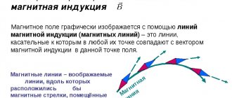
Magnetic field circulation theorem
The circulation of the magnetic field of direct currents along any closed circuit is proportional to the sum of the current strengths penetrating the circulation circuit.
The circulation theorem states that the circulation of vector B of the magnetic field of direct currents along any circuit L is always equal to the product of the magnetic constant μ0 by the sum of all currents passing through the circuit:
The circulation of the magnetic induction vector B along a given contour is called the integral
Maxwell's system of equations.
Maxwell's equations are a system of equations in differential or integral form that describe the electromagnetic field and its relationship with electric charges and currents in vacuum and continuous media. Together with the expression for the Lorentz force, which specifies the measure of the influence of the electromagnetic field on charged particles, they form a complete system of equations of classical electrodynamics, sometimes called the Maxwell-Lorentz equations.
Differential form
Maxwell's equations are represented in vector notation by a system of four equations, which is reduced in component representation to eight (two vector equations contain three components each plus two scalar) linear partial differential equations of the first order for 12 components of four vector functions ( ):
| Name | GHS | SI | Example verbal expression |
| Gauss's law | Electric charge is the source of electrical induction. | ||
| Gauss's law for magnetic field | There are no magnetic charges | ||
| Faraday's Law of Induction | A change in magnetic induction generates a vortex electric field. | ||
| Magnetic field circulation theorem | Electric current and changes in electrical induction generate a vortex magnetic field |
In the following, bold font denotes vector quantities, and italics indicate scalar quantities.
Introduced designations:
· - density of external electric charge (in SI units - C/m³);
· - electric current density (conduction current density) (in SI units - A/m²); in the simplest case - the case of a current generated by one type of charge carriers, it is expressed simply as , where is the (average) speed of movement of these carriers in the vicinity of a given point, is the charge density of this type of carriers (in the general case it does not coincide with )[29] ; in the general case, this expression must be averaged over different types of media;
· — speed of light in vacuum (299,792,458 m/s);
· — electric field strength (in SI units — V/m);
· — magnetic field strength (in SI units — A/m);
· - electrical induction (in SI units - C/m²);
· — magnetic induction (in SI units — T = Wb/m² = kg•s−2•A−1);
· is a differential operator, in this case:
means vector rotor,
means vector divergence.
Integral form
Using the Ostrogradsky-Gauss formula and Stokes' theorem, Maxwell's differential equations can be given the form of integral equations:
| Name | GHS | SI | Example verbal expression |
| Gauss's law | The flow of electrical induction through a closed surface is proportional to the amount of free charge located in the volume that surrounds the surface. | ||
| Gauss's law for magnetic field | The flux of magnetic induction through a closed surface is zero (magnetic charges do not exist). | ||
| Faraday's Law of Induction | The change in the flux of magnetic induction passing through an open surface, taken with the opposite sign, is proportional to the circulation of the electric field on a closed loop, which is the boundary of the surface. | ||
| Magnetic field circulation theorem | The total electric current of free charges and the change in the flow of electrical induction through an open surface are proportional to the circulation of the magnetic field on a closed loop, which is the boundary of the surface. |
Introduced designations:
· - a two-dimensional closed surface in the case of the Gauss theorem, limiting the volume, and an open surface in the case of the Faraday and Ampere-Maxwell laws (its boundary is a closed contour).
· - electric charge contained in a volume limited by the surface (in SI units - C);
· - electric current passing through the surface (in SI units - A).
When integrating over a closed surface, the vector of the area element is directed outward from the volume. The orientation when integrating over an open surface is determined by the direction of the right-hand screw, which is “screwed in” when turning in the direction of traversing the contour integral over .
Simplified approach
It is quite difficult to express the law in differential representation. Additional components will need to be introduced. It is necessary to take into account the influence of molecular currents. The presence of eddy currents causes the formation of a magnetic eddy field within the circuit.
The electric displacement vector is comparable to the intensity vector of the present magnetic field H. In this case, the orientation of the displacement vector depends on the rate of change of magnetic induction.
To simplify calculations in practice, formulas of the law for the magnetic field of total currents are often used, presented as a summation of extremely small sections of the circuit, taking into account the influence of eddy fields. When implementing this method, the contour is mentally divided into infinitesimal segments. On these segments, the conductors are considered to be straight, and the magnetic field in such sections of the circuit is considered uniform.
In one discrete section, the tension vector Um is determined by the formula: Um= HL×ΔL, where HL is the circulation of the tension vector in the ΔL section of the contour L. Then the total tension UL along the entire contour is calculated by the formula: UL= Σ HL× ΔL .
Circulation of a vector field. Stokes formula
| Site Map |
The final lesson on the basics of vector analysis will be devoted to another characteristic of a vector field called circulation. What do we associate this term with at the layman level? Air circulation, liquid circulation in some system; Moreover, the Latin root of this word (circulare) tells us that the process goes “in a circle.”
That's right, the concept of circulation came to field theory from a hydrodynamic problem, where it was necessary to estimate the movement of a fluid along a closed loop. Let's build the simplest model: let a liquid circulate in a certain closed pipe, and its movement is described by a velocity field . Consider an arbitrary closed streamline. To simplify, we will assume that each point on the line corresponds to a field vector protruding from it, which shows the direction and speed of fluid movement at a given point.
Circulation () of a vector field along a contour is a scalar quantity , numerically equal to the curvilinear integral of the 2nd kind along this contour:
According to the general principle of integration , this integral combines the projections of vectors “sticking out” from the contour onto the coordinate axes along all infinitesimal pieces of the contour, which is an estimate of the movement of the fluid. And directly from the integral it is clear that circulation depends on two things:
– the length of the circuit itself (the longer, the greater the circulation);
– flow velocity * (the longer the “ef” vectors, the larger their infinitesimal projections and the greater the value).
* Over time, the concept of circulation extended to an arbitrary vector field, where there is literally nothing to circulate
In this case, the contour can obviously be bypassed in two ways: in one direction or in the opposite direction. In both cases, the same absolute value of circulation will be obtained with different signs (unless, of course, ). In practice, a counterclockwise bypass is more often used - when for a person “walking along the contour” the area limited by the contour remains on the left hand. This direction of traversal is called positive.
It should also be noted that the requirement for a closed loop is not mandatory - circulation can also be calculated using an arbitrary piecewise smooth line, which allows for seamless integration. However, historically and methodologically it has developed that in practical problems the circuit is, as a rule, closed.
And, if we write out the curvilinear circulation integral for a vector field in detail, then its physical meaning will “reveal” to us:
Namely, circulation is equal to the work of a vector field along a closed loop, which I also mentioned in the first lesson on field theory . This meaning is more typical for force fields, but in the hydrodynamic model the result can be interpreted as the work of the velocity field in moving a material point.
Thus, today we will have two tasks “in one bottle”! In addition, we almost never solved curvilinear integrals over spatial contours, and now is the time to catch up:
Example 1
Calculate the circulation of the vector field along the triangle in the positive direction.
Solution : draw a triangle in the drawing and be sure to mark with arrows the order in which it is traversed:
The circulation of a vector field along a closed contour is equal to a curvilinear integral of the 2nd kind along a given contour, and due to the additivity property:
As they say, divide and conquer:
1) Let's calculate the circulation along the segment:
Using the points and we will find the directing vector of the straight line: , and since its “zeta” coordinate is equal to zero, the canonical equations of the straight line take the following form: . We mentally check that the coordinates of points “a” and “be” satisfy the resulting equations. Since , then we have the opportunity to reduce the curvilinear integral to a definite integral with integration along the “x” or “y”. From the left proportion we express: and find the differential: - thus the solution is reduced to the variable “x”, which, in accordance with the direction of integration , changes ( look at the drawing! ) from 3 to 1:
Alternatively, from the equations of the straight line you can express, find and integrate over the “y” from 0 to 2. Let’s not miss an excellent opportunity to check:
2) Let us calculate the circulation of the vector field along the segment:
We will find the direction vector of the corresponding straight line at the points : – and since all its coordinates are non-zero, we will not be able to “zero” any variable in the curvilinear integral. What to do? Let's write down the parametric equations of the straight line - by point (it is more convenient to take the beginning of the path) and by the direction vector: It is easy to see that the beginning of the segment corresponds to the value , and the end to the value . All that remains is to find the differentials of the parametric equations: and CAREFULLY substitute all the belongings:
3) And finally, let’s calculate the circulation of the field along the segment:
Since the path lies in the plane, the “Y” coordinate will be equal to zero, which allows us to reduce the solution to a definite integral along “X” or “Z”. Let’s compose the canonical equations of a straight line using a point and a direction vector: – do not forget to mentally check that the coordinates of the points satisfy the resulting equations.
From the proportion it is easier to express, find and integrate along “zet” ( attention! ) from 2 to 0 - strictly in the direction of traversal:
Don’t let your soul be lazy - now let’s express, find and integrate over “x” from 0 to 3: , which is what we needed to check.
By the way, both in the first and in this paragraph you can use parametric equations - whichever is more convenient for you.
Thus, the circulation of a vector field along a closed loop:
Answer:
Most likely, this result is not very clear to you from the point of view of hydrodynamics, and a little later I will explain its meaning. But first, let’s answer the old sacramental question: couldn’t it be simpler?
Stokes formula
The circulation of a vector field along a closed contour is equal to the flux of its rotor through a surface stretched over a given contour in the direction that corresponds to the direction of bypassing the contour:
namely, if we look at the surface from the tip of its normal vectors (vectors), then the path along the contour should be VISIBLE TO US as being carried out COUNTERclockwise. Look at the triangle (drawing above) from the side of the tip of the unit normal vector. Is the circuit traversed counterclockwise? Yes * . This means that this is the required normal vector, and therefore we should calculate the surface integral over the upper side of the triangle.
* Look at the situation from the other side of the triangle
According to the Stokes formula:
, where is the unit normal vector of the upper side of the triangle.
Note : in fact, on the right side there is a surface integral of the 2nd kind - already reduced to a surface integral of the 1st kind
Let's find the rotor function of the field. To avoid confusion, let’s write out the field components and take partial derivatives in “rotary” order:
Thus: therefore, our field is potential and:
Well, of course - if we remember the physical meaning of circulation (the work of a vector field along a contour), and remember that the work along a closed contour in a potential field is equal to zero, then everything falls into place.
Thus, the circulation of the vector field is zero not only along the triangle, but in general along any closed contour of space. From which the hydrodynamic meaning of the problem becomes clear: imagine that the triangle is inside a closed pipe. Since the velocity field is potential, the circulation will be zero not only along this triangle, but also along any internal closed line. This tells us that the movement of liquid in the pipe is multidirectional and compensated - as much as it circulates in one direction, so much circulates in the other.
In fact, we have used the Stokes formula before: if the contour lies entirely in the plane, then we get its special case called Green’s formula :
, where is a closed area bounded by the contour . And in fact, now we have solved the spatial analogue of Example 12 of lesson Curvilinear integrals along a closed contour .
It is interesting to note that the field considered in the problem is not only potential , but also solenoidal :
Such fields (both potential and solenoidal) are called harmonic. And under this term I always imagine a full-flowing, wide river with a smooth flow, along which a whole flotilla of boats floats majestically, without the slightest deviation from the straight course. And there really is some kind of bewitching harmony in this. However, this is only an association - come up with a “stormy” example yourself
In the vector analysis course, there is a whole section devoted to harmonic fields, but now we are returning to practical matters, and for your own solution, I offer you a similar problem:
Example 2
Calculate the circulation of the vector field along the triangle in the positive direction in two ways: a) directly, b) using the Stokes formula.
This is a more common case, where all the segments lie in coordinate planes, and therefore here you can use exclusively Cartesian coordinates. However, parametric equations are also a good option, because there is only one letter =) - the main thing is to correctly understand the limits of parameter change.
When using the Stokes formula, we do not get confused - it calculates the flow NOT of the field ITSELF, but of its rotor . And yes, here you will need to create an equation of the plane .
DO NOT BE LAZY and be sure to solve this task! It may not be very interesting from the point of view of content, but it is extremely useful for developing techniques for solving curvilinear integrals . At the end of the lesson, you can familiarize yourself with a sample solution and some rational calculation techniques that allow you to minimize labor costs and reduce the risk of errors.
In addition to the triangle contour, perhaps the only more popular is the circle :
Example 3
Calculate the circulation of a vector field along a closed loop directly and using the Stokes formula
Solution : the proposed equations define a circle lying in the plane , radius 2, centered on the axis. Moreover, the condition does not say anything about the order of traversing the contour, and we, in principle, can choose any of them. Let's go the “traditional” way:
1) Let's calculate the work of the vector field directly. With “X”, “Y”, “Z” and their differentials, everything is transparent here: all that remains is to control the limits of parameter change: – if , then – the white point of the contour (see drawing); – if , then – the highest point of the contour. Thus, when changing, the circle is "drawn" in the opposite direction with respect to our traversal order, and therefore the integral should be taken from to 0:
We use trigonometric formulas :
Answer:
The negative sign tells us that the circulation is carried out (completely or predominantly) against the traversal order we have chosen, and if we walked around the circle in the opposite direction, it would turn out
2) Let us calculate the circulation using the Stokes formula:
Let's find the rotor function:
Since the surface stretched over the contour is a flat figure (circle), then for all its points the unit normal vector can “look” only in two directions. Which vector to choose: or ? Let us remember the rule: from the tip of the vector, the circuit traversal should be VISIBLE TO US counterclockwise. The vector satisfies this condition. Be sure to look at the circle from the other side - from this point of view, the circuit is traversed clockwise, and therefore the vector is not suitable.
Let's find the scalar product :
Now we charge the Stokes formula:
Here you can refer to the fact that the integral is equal to the area of the circle: and immediately give the answer, but we will go the academic route.
Since the surface is “fully” projected only onto the plane, then there is nothing left but to apply the particular formula . I especially emphasize that this is a special case, and if there were at least some variables under the integral, then the full version would be required
But with us everything is simpler:
And here again we can refer to the fact that the resulting double integral is numerically equal to the area of a circle of the same radius, but I will “finish” the integral with the help of an “exotic” transition to polar coordinates in the plane. With the order of traversal, everything is clear here: – note that the polar angle changes in the standard direction, from the semi-axis towards the semi-axis. Roughly speaking, the role of the “y” here is played by the “ze” variable, which means:
Answer:
If you choose a different direction to go around the circle, you will have to use the oppositely directed vector, which will obviously change the sign. However, a negative sign is no worse than a positive one and only indicates that we have calculated the circulation completely or predominantly “against the flow.”
A couple of problems to solve on your own. Simpler:
Example 4
Calculate the circulation of a vector field along a closed contour directly and using the Stokes formula. Select the positive direction of the bypass.
In the example I gave a scrupulous solution, but in practice you can also use the geometric meaning of integrals; usually teachers are loyal to this.
And a more interesting problem:
Example 5
Find the modulus of circulation of the vector field along the contour
The contour here represents the line of intersection of the cylinder and the plane , namely, an ellipse ; and, by the way, in the lesson on triple integrals in Example 7, I talked about how to construct such a section. It is interesting to note that here you can easily do without a drawing, since you need to find the absolute value of the circulation, the direction of the bypass does not matter - we simply stupidly integrate over “te” from 0 to . With the parametric equations of the “oblique” ellipse, I think there should be no problems. But this is a double-edged sword - you may find the second solution easier.
There are more complex tasks, but for the purposes of this lesson this will be enough, because simpler is better - and more understandable. In addition, I have not told everything on the topic, in particular that the very concept of a rotor is defined through circulation and a surface stretched over a contour + another interesting point that concerns the surface. Read, for example, the 3rd volume of Fichtenholtz.
Well, I congratulate you on successfully completing an entertaining course on field theory . I hope it was clear, interesting and useful, and now no one will be afraid, at least, of the fancy notations in textbooks.
All that remains to be done is to hand you a shovel and send it to the vast field of vector analysis =) Additional problems with solutions are in the corresponding archive of the solution bank , the mathprofi.com , or in this workbook. Just be careful and critical - shortcomings and errors can be anywhere.
I wish you success!
Solutions and answers:
Example 2: Solution : let's depict the integration contour in the drawing: a) Let's solve the problem directly:
1) Let's calculate the circulation along the segment. Since , then: Let’s compose the equations of a straight line using a point and a direction vector: , from which we express: In this case, it changes from 0 to 3: Check the solution in another way!
2) Let us calculate the circulation of the field along the segment. Since , then: Let’s compose the equations of a straight line using a point and a direction vector: , from where: Let’s find the differential: varies from 3 to 0: Solve it yourself using the variable “zet”
3) Let us calculate the circulation of the field along the segment. Since , then: Let’s compose the equations of a straight line using a point and a direction vector: In this case, it is more advantageous to express it varies from 3 to 0:
Thus, circulation in a closed loop:
Answer:
b) Let's calculate the circulation of the vector field using the Stokes formula: Let's find the rotor of the vector field: . In this case: Thus: Let's create an equation of the plane using a point and vectors: Let's write down the normal vector of this plane: and find the corresponding unit vector: Note : from the tip of this vector, the circuit is visible to us counterclockwise, therefore, this is the desired normal vector Let's find scalar product: Thus: To calculate the surface integral of the 1st kind, we use the formula , where is the projection of the triangle onto the plane. In this case: The double integral is numerically equal to the area of the triangle:
Answer:
Example 4: Solution : draw: 1) Calculate the work of the vector field directly: Thus:
2) Let us calculate the circulation using the Stokes formula: , where is the surface spanned by the contour Find . In this case: Dot product: Thus: Project the surface onto the plane and use the formula , where is the projection of the surface. In this case: Let's move on to polar coordinates in the plane:
Answer:
Example 5: Solution : write the parametric equations of the cylinder: (any real number ) Substitute the first two equations into the equation of the plane: Thus, the section of the cylinder by the plane (ellipse) is determined by the equations: Let's find the differentials: and calculate the circulation of the vector field along the contour Г in the direction that corresponds to a change in the parameter within:
It is, of course, more convenient to carry out simplifications and calculate integrals separately =)
Answer:
Try to arrive at the same result using the Stokes formula.
Author: Emelin Alexander
Higher mathematics for correspondence students and more >>>
(Go to main page)
How can you thank the author?
Zaochnik.com – professional help for students
15% discount on your first order, when placing your order, enter promotional code: 5530-hihi5
Law in integral representation
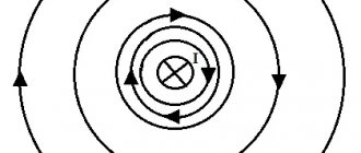
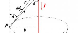
Let us consider an infinitely straight conductor through which an electric current circulates, forming a field limited by a contour in the form of a circle. The plane piercing the conductor is a circle outlined by the line of a given circle (see Fig. 1).
Rice. 1. Field of infinite forward current
We will use the method of dividing the contour into tiny sections dl (elementary vectors of the contour length). Let φ be the angle between the vectors dl and B. In our case, when summing the segments, the induction vector B is rotated so that it outlines a circle, that is, the angle φ → 2π.
The formula follows from the Ostrogradsky-Gauss theorem:
Considering that cos φ = 1,
hence:
This formula is a postulate confirmed experimentally. According to this postulate, the circulation of vector B around a circle, that is, along a closed contour, is equal to μ0I, where μ0 = 1/c2 ε0 is the magnetic constant.
The orientation of the dB vector is determined by applying the gimlet rule. This direction is always perpendicular to the density vector. If there are several conductors (for example, N), then
Each current, taking into account its sign, must be taken into account the number of times that corresponds to the number of its circuits.
The current is taken with a “+” sign if it forms a right-handed system in the direction of bypass. In this case, the current in the opposite direction is considered negative.
Note that the formula is valid only for vacuum. Under normal conditions, it is necessary to take into account the permeability of the medium.
If the current is distributed in space (arbitrary current), then
where S is the surface stretched over the contour, j is the volumetric current density. Taking into account the last expression, the formula for the total current in vacuum can be written:
Rice. 2. Illustration of the law for vacuum
It follows from this:
- The law is valid not only for an infinitely straight conductor, but also for circuits of arbitrary configuration.
- The circulation of the magnetic induction vector B, oriented along the magnetic lines, is always different from zero.
- Non-zero circulation indicates that the magnetic field of a straight, infinitely long conductor is not potential. Such a field is called a vortex or solenoid field.
Circulation and flux of magnetic induction vector
The circulation and flow of the magnetic induction vector (as well as any vector in general) are determined in the same way as for the electric field strength vector.
Circulation along a straight segment of a homogeneous field
is called the scalar product: , where is the angle between the vectors and .
Let's consider a section of an arbitrary directed curve. Let's divide this section into small segments directed in the same way as the curve itself. Then, the circulation of a vector along a section of a curve is called a curvilinear integral, which represents the limit of the sum when dividing the curve into infinitesimal segments:
.
A small section of the curve can be considered a straight segment, and the field within this section can be considered homogeneous, therefore each term in the sum represents the circulation of the vector along the segment.
Vector circulation in a closed loop
we will denote the curve as .
Magnetic flux
vector in a uniform field through a flat surface of area is called the quantity
, (3.19)
where is the unit vector of the normal to the surface, is the angle between the direction of the vector and the direction of the normal to the surface. The SI unit of magnetic flux is Weber
(Wb).
Now consider a section of an arbitrary surface. The flow of a vector through a section of a surface is called a surface integral, which is the limit of the sum when dividing the surface into pieces of infinitesimal areas:
. (3.19a)
A small area of the surface can be considered flat, and the field within this area can be considered homogeneous, therefore each term in the sum represents the vector flow through the flat surface.
Vector flow through a closed loop
the surface will be denoted as .
Let us formulate two theorems about the circulation and flow of the magnetic induction vector.
Theorem on the circulation of the magnetic induction vector
(for a field in vacuum). Circulation of the magnetic induction vector along an arbitrary closed directional contour:
, (3.20)
where is the algebraic sum of currents passing through an arbitrary surface stretched over the contour along which the circulation is calculated. The direction of traversing the contour and the direction of the normal to the surface stretched over it are related by the gimlet rule. If the current flows in the direction of the normal, then it should be considered positive, if on the contrary - negative.
For example, the circulation of the magnetic induction vector along the contour shown in Fig. 3.14, is equal to .
Theorem on the flux of the magnetic induction vector.
The flux of the magnetic induction vector through an arbitrary closed surface is zero:
. (3.21)
It is useful to compare theorems on the circulation and flow of the magnetic induction vector with the corresponding theorems for the electric field strength vector. Let us recall the theorem about the flow of the electric field strength vector (Gauss’s theorem, see formula 1.18):
.
The meaning of this theorem is that the sources of the electric field are electric charges. They create the flow of the electric field strength vector. Lines of force begin at charges and end at them. And the meaning of the theorem about the flux of the magnetic induction vector is that magnetic charges do not exist in nature. Therefore, magnetic lines of force do not begin or end anywhere, they are closed. This means that the flux of the magnetic induction vector through any closed surface is equal to zero (the number of lines that enter inside the surface is the same that will come out).
The circulation of the electric field strength vector along any closed loop is zero (equation 1.34):
.
The meaning of this equation is that the electric field created by any system of charges is a potential field (for more details, see section 1.12). An electric field, in addition to tension - a force characteristic, also has an energy characteristic - potential. The circulation theorem for the magnetic induction vector says that the sources of the magnetic field are electric currents (essentially moving electric charges), which create the circulation of the vector. In addition, since the circulation of the magnetic induction vector along a closed loop can be different from zero, the magnetic field is a non-potential field. Fields with closed lines of force are called vortex or solenoidal. This is what a magnetic field is.
Let us give several examples of the application of the circulation theorem for a magnetic field.
Example 3.6. Determine the magnetic field created by a straight infinitely long conductor carrying current.
Solution. As an arbitrary closed contour, we choose a circle with radius , the center of which is on the axis of the wire (such a contour will coincide with one of the power lines - see Fig. 3.13, a). In this case, the scalar product is . Since the circuit is penetrated by only one current, using the circulation theorem for the magnetic field we obtain:
.
The magnitude of the vector is the same at all points of the contour, therefore, as a constant, it can be taken out of the integral sign:
.
The integral is simply the length of the contour. Thus,
,
from where we find the magnitude of the magnetic field at a distance from the wire:
.
The last expression exactly coincides with the result obtained in example 3.3 (see formula 3.14) from the Biot-Savart-Laplace law.
Note that formula 3.14 can also be used in the case of a conductor of finite dimensions when calculating the field approximately opposite the central part of the conductor at points located from it at distances much shorter than the length of the conductor.
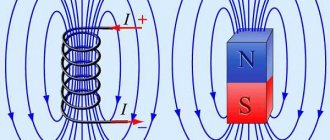
Example 3.7. Find the magnetic field inside the solenoid with length, number of turns and current.
Solution. As a bypass contour, we choose a rectangular ACDE
(see Fig. 3.15) so that segment
AC
approximately lies in the middle part of the solenoid, and segment
DE
is located at a large distance from the solenoid. According to the circulation theorem for the magnetic field, we have:
.
By placing a small magnetic needle at various points in space, it can be shown that the magnetic field in the middle part of the solenoid, both outside and inside, is directed parallel to the axis of the solenoid. Consequently, on contour segments CD
and
EA
dot product
,
and on the segment AC
:
.
Thus, the circulation of the magnetic field along segments CD
and
EA
are equal to zero:
, ,
and along the segment AC
:
(here the magnitude of the magnetic induction vector is taken out of the integral sign, since it must be constant on the segment AC
due to the axial symmetry of the system).
At a large distance from the solenoid, the value of magnetic induction is close to zero, therefore the circulation of the magnetic field along the segment DE
is equal to zero:
.
As a result we get:
Sum of currents passing through the ACDE
:
,
where is the number of turns piercing the ACDE
(in Fig. 3.15 these turns are shown) is the number of turns per unit length of the solenoid. Then:
.
If the number of turns per unit length of the solenoid is represented as , where is the total number of turns, and is the length of the solenoid, then:
.
The result obtained coincides with formula (3.18) for the field on the axis of an infinitely long solenoid. Using the circulation theorem, we showed that in the case of a sufficiently long solenoid, the result (3.18) can be used to calculate the field at any point inside the solenoid in its middle part, and not just on the axis.
The circulation and flow of the magnetic induction vector (as well as any vector in general) are determined in the same way as for the electric field strength vector.
Circulation along a straight segment of a homogeneous field
is called the scalar product: , where is the angle between the vectors and .
Let's consider a section of an arbitrary directed curve. Let's divide this section into small segments directed in the same way as the curve itself. Then, the circulation of a vector along a section of a curve is called a curvilinear integral, which represents the limit of the sum when dividing the curve into infinitesimal segments:
.
A small section of the curve can be considered a straight segment, and the field within this section can be considered homogeneous, therefore each term in the sum represents the circulation of the vector along the segment.
Vector circulation in a closed loop
we will denote the curve as .
Magnetic flux
vector in a uniform field through a flat surface of area is called the quantity
, (3.19)
where is the unit vector of the normal to the surface, is the angle between the direction of the vector and the direction of the normal to the surface. The SI unit of magnetic flux is Weber
(Wb).
Now consider a section of an arbitrary surface. The flow of a vector through a section of a surface is called a surface integral, which is the limit of the sum when dividing the surface into pieces of infinitesimal areas:
. (3.19a)
A small area of the surface can be considered flat, and the field within this area can be considered homogeneous, therefore each term in the sum represents the vector flow through the flat surface.
Vector flow through a closed loop
the surface will be denoted as .
Let us formulate two theorems about the circulation and flow of the magnetic induction vector.
Theorem on the circulation of the magnetic induction vector
(for a field in vacuum). Circulation of the magnetic induction vector along an arbitrary closed directional contour:
, (3.20)
where is the algebraic sum of currents passing through an arbitrary surface stretched over the contour along which the circulation is calculated. The direction of traversing the contour and the direction of the normal to the surface stretched over it are related by the gimlet rule. If the current flows in the direction of the normal, then it should be considered positive, if on the contrary - negative.
For example, the circulation of the magnetic induction vector along the contour shown in Fig. 3.14, is equal to .
Theorem on the flux of the magnetic induction vector.
The flux of the magnetic induction vector through an arbitrary closed surface is zero:
. (3.21)
It is useful to compare theorems on the circulation and flow of the magnetic induction vector with the corresponding theorems for the electric field strength vector. Let us recall the theorem about the flow of the electric field strength vector (Gauss’s theorem, see formula 1.18):
.
The meaning of this theorem is that the sources of the electric field are electric charges. They create the flow of the electric field strength vector. Lines of force begin at charges and end at them. And the meaning of the theorem about the flux of the magnetic induction vector is that magnetic charges do not exist in nature. Therefore, magnetic lines of force do not begin or end anywhere, they are closed. This means that the flux of the magnetic induction vector through any closed surface is equal to zero (the number of lines that enter inside the surface is the same that will come out).
The circulation of the electric field strength vector along any closed loop is zero (equation 1.34):
.
The meaning of this equation is that the electric field created by any system of charges is a potential field (for more details, see section 1.12). An electric field, in addition to tension - a force characteristic, also has an energy characteristic - potential. The circulation theorem for the magnetic induction vector says that the sources of the magnetic field are electric currents (essentially moving electric charges), which create the circulation of the vector. In addition, since the circulation of the magnetic induction vector along a closed loop can be different from zero, the magnetic field is a non-potential field. Fields with closed lines of force are called vortex or solenoidal. This is what a magnetic field is.
Let us give several examples of the application of the circulation theorem for a magnetic field.
Example 3.6. Determine the magnetic field created by a straight infinitely long conductor carrying current.
Solution. As an arbitrary closed contour, we choose a circle with radius , the center of which is on the axis of the wire (such a contour will coincide with one of the power lines - see Fig. 3.13, a). In this case, the scalar product is . Since the circuit is penetrated by only one current, using the circulation theorem for the magnetic field we obtain:
.
The magnitude of the vector is the same at all points of the contour, therefore, as a constant, it can be taken out of the integral sign:
.
The integral is simply the length of the contour. Thus,
,
from where we find the magnitude of the magnetic field at a distance from the wire:
.
The last expression exactly coincides with the result obtained in example 3.3 (see formula 3.14) from the Biot-Savart-Laplace law.
Note that formula 3.14 can also be used in the case of a conductor of finite dimensions when calculating the field approximately opposite the central part of the conductor at points located from it at distances much shorter than the length of the conductor.
Example 3.7. Find the magnetic field inside the solenoid with length, number of turns and current.
Solution. As a bypass contour, we choose a rectangular ACDE
(see Fig. 3.15) so that segment
AC
approximately lies in the middle part of the solenoid, and segment
DE
is located at a large distance from the solenoid. According to the circulation theorem for the magnetic field, we have:
.
By placing a small magnetic needle at various points in space, it can be shown that the magnetic field in the middle part of the solenoid, both outside and inside, is directed parallel to the axis of the solenoid. Consequently, on contour segments CD
and
EA
dot product
,
and on the segment AC
:
.
Thus, the circulation of the magnetic field along segments CD
and
EA
are equal to zero:
, ,
and along the segment AC
:
(here the magnitude of the magnetic induction vector is taken out of the integral sign, since it must be constant on the segment AC
due to the axial symmetry of the system).
At a large distance from the solenoid, the value of magnetic induction is close to zero, therefore the circulation of the magnetic field along the segment DE
is equal to zero:
.
As a result we get:
Sum of currents passing through the ACDE
:
,
where is the number of turns piercing the ACDE
(in Fig. 3.15 these turns are shown) is the number of turns per unit length of the solenoid. Then:
.
If the number of turns per unit length of the solenoid is represented as , where is the total number of turns, and is the length of the solenoid, then:
.
The result obtained coincides with formula (3.18) for the field on the axis of an infinitely long solenoid. Using the circulation theorem, we showed that in the case of a sufficiently long solenoid, the result (3.18) can be used to calculate the field at any point inside the solenoid in its middle part, and not just on the axis.
Environmental influence
The result of the interaction of magnetic fluxes and direct currents is influenced by the environment. Substances have magnetic permeability in the flow of the induction vector, which makes adjustments to the interaction of the magnetic environment with conduction currents. In a homogeneous isotope medium, where the value of the electromagnetic induction vector is the same at all points, vectors B and H are related to each other by the following relationship:
where H is the magnetic field strength, and the symbol μ denotes magnetic permeability.
Electric charge carriers create their own microcurrents. The circulation of the vector characterizing the electrostatic field is always zero. Therefore, electrostatic fields, unlike magnetic fields, are potential.
Vector B displays the resulting value of the macro- and microcurrent fields. Electrostatic induction lines always remain closed, including those on positive charges.
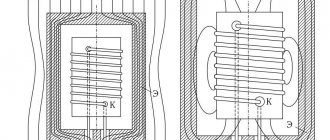
Rice. 3. Law of total current in matter
For fields that operate in a medium consisting of different substances, it is necessary to take into account microcurrents characteristic of specific structures that form this medium.
The statement stated above is true for the fields of solenoids or any other structure that has the properties of finite magnetic permeability.
Integral formula for total current
To formulate the law, you need to imagine a closed loop, inside which there are one or more wires through which electric current passes. The contour can have any shape, but it must be closed. To make calculations, it is necessary to divide the curve into elementary sections that are so small that they can be considered straight segments with minimal error.
In this case, using the gimlet rule, you can determine the direction of the magnetic field strength created by each conductor on each elementary segment. To obtain the total result, you will need to integrate along the contour.
The integral formula for the total current law is as follows:
Given the expression
the formula can be written like this:
It is a postulate confirmed experimentally. According to it, the circulation of the magnetic induction vector in a closed loop is equal to μ0I, where μ0 is the magnetic constant.
The theorem on the circulation of the magnetic induction vector is based on the Biot-Savart law and the principle of magnetic field superposition. In general, it has the following formulation:
For an arbitrary current (distributed in space), the following equality is true:
Taking into account this equality, the formula for the total current in vacuum takes the following form:
On the left side, integration along the contour of the magnetic induction vector is used. The right side considers the sum of the currents passing inside the circuit, multiplied by the magnetic constant.
The interaction of electric currents and magnetic fluxes depends on the environment in which they reside. In addition, different substances have different magnetic permeability. Taking this into account, the law of total current for the magnetic field in a substance is expressed by the following formula:
Thoroid
In electrical engineering, you often have to deal with coils of different types and sizes. A coil formed by turns wound on a toroidal (donut-shaped) core is called a toroid. Important characteristics of the torus core are its radii - internal (R1) and external (R2).
The field inside the solenoid at a distance r from the center is equal to:
conclusions
Based on the above, we come to the conclusion:
- The law of total current establishes the relationship between the strength of the magnetic field and the movement of electric charges in this field.
- The law applies to all environments, subject to permissible current densities.
- The law is also true in the fields of permanent magnets.
When calculating, it does not matter what formula we use - the essence of the law remains unchanged: it expresses the interactions that occur between currents and the magnetic fields they create that penetrate a closed circuit.
The conclusions of the law are taken into account when designing electromagnetic devices. The presence of turbulence in electromagnetic fields leads to a decrease in efficiency. In addition, vortex fields negatively affect the performance of electronic elements located in the area of their action.
Designers of electrical devices strive to minimize such influences. For example, instead of conventional solenoids, toroidal coils are used, outside of which there are no electromagnetic fields.
Solving problems in TOE, OTC, Higher Mathematics, Physics, Programming...
The proven circulation theorem applies to any case of a magnetic field, provided that it is created by direct currents. It is also true in the presence of a magnet in which bound currents arise in the presence of an external field. In this case, the right side of the equation for the circulation of vector B must include both free and bound currents. Let's consider this case. Let a conductor with current be placed in a magnet (Fig. 3.30). A magnet can be inhomogeneous and have boundaries (we are considering the general case). What is the circulation of the magnetic field induction vector along contour L? It is proportional to the sum of the currents coupled to the circuit. In addition to the current J, it is necessary to take into account the associated currents of the magnetic molecules. We liken molecules to magnetic dipoles. Only some of the dipole molecules are strung on the circuit. These dipoles seem to form a kind of tube, along the surface of which current flows. The equation for the circulation of vector B will have the form:(3.54)
The second term on the right represents the bound current coupled to the loop. It can be represented in the form of a certain integral. Let us introduce the linear density of the surface current on the tube (j'). This is the current strength per unit length of the tube. Then the current strength per element of tube length d will be equal to j'd. The current flowing over the surface of the entire tube is determined by the integral
Consequently, the equation for circulation will take the form:
(3.55)
Now you can use formula (3.44), which connects the current density on the surface of the tube with the magnetization vector. The equation for circulation will be rewritten in the form
(3.56)
Let's transform it a little:
(3.57)
Here it is taken into account that M cos a dl = Mdl, and that in the general case more than one free current can be coupled to the circuit. Vector
(3.58)
called magnetic field strength. With the introduction of such a concept, the circulation theorem will be formulated in the form of the following relation:
(3.59)
The circulation of the magnetic field strength vector is equal to the sum of free currents associated with the circuit. Bound currents, thanks to the introduction of the concept of magnetic field strength vector, are not explicitly included in the equation for circulation. This is the meaning of introducing a new concept - magnetic field strength. It is introduced from purely formal, calculated, considerations, from considerations of convenience. The concept of magnetic field strength has no physical meaning. This can be seen from its definition (3.58). The field strength vector essentially represents the difference between two vectors: magnetic field induction and magnetization of the magnet. But these two vectors characterize completely different physical entities: the first is a characteristic of the field, and the second is a characteristic of matter. It is possible to find some formal interpretations for the vector H, but they cannot give any physical meaning to this quantity. The magnetization vector M is determined by the induction of the field B in the magnet. In isotropic para- and diamagnets, this vector is proportional to the vector B. Then from formula (3.58) it follows that for these substances the vector M will also be proportional to the vector H. It is this dependence of M on H (and not the dependence of M on B) that is taken in practice as basis, i.e. the law for the magnetization vector is written in the following form:
M = cH
(3.60)
(c > 0 for paramagnetic materials and c < 0 for diamagnetic materials)
The proportionality coefficient in this formula is called magnetic susceptibility. For para- and diamagnets it does not depend on H, and it makes sense to introduce it as an independent concept. Then, according to formula (3.58) for vector B, we obtain the following expression:
(3.61)
The factor 1+c=m is called magnetic permeability, and the resulting relationship between B and H is rewritten as
B = mm0N (in SI)
(3.62)
In para- and diamagnets there is a constant quantity that completely characterizes the substance, and this, as for , fully justifies its introduction into physics. In ferromagnets it is determined not only by the properties of the substance, but is also a function of the field, which imposes an element of convention on the concept of magnetic permeability of a ferromagnet. Let us illustrate the convenience of introducing the concept of magnetic field strength using the example of a solenoid. If the solenoid has a core (for example, iron), then the formula for the induction of field B is:
B = m(H)m0nJ
(3.63)
In this formula, the dependence (H) can be determined (and not easily!) only empirically. But for vector H the formula has a simple form:
H = nJ
The magnetic field strength is equal to the product of the number of turns per unit length of the solenoid and the current strength. Thus, measuring H is not difficult. In conclusion, let us note that in electrostatics we also had to introduce two field characteristics: strength and electrical displacement - E and D. The relationship between them is similar to relationship (3.62):
D = ee0E.
(3.64)
But in their meaning, formulas (3.64) and (3.62) are significantly different: in electrostatics, the voltage vector has a physical meaning, and the electric displacement vector is an auxiliary, artificial quantity. In magnetic field theory it is the other way around: the magnetic induction vector has a physical meaning, and intensity is an artificial concept.