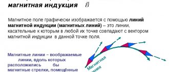
Good day to all. In the last article I talked about the magnetic field and dwelled a little on its parameters. This article continues the topic of the magnetic field and is devoted to such a parameter as magnetic induction. To simplify the topic, I will talk about the magnetic field in a vacuum, since different substances have different magnetic properties, and as a result, it is necessary to take their properties into account.
To assemble a radio-electronic device, you can pre-make a DIY KIT kit using the link.
Biot–Savart–Laplace law
As a result of studying the magnetic fields created by electric current, researchers came to the following conclusions:
- magnetic induction created by electric current is proportional to the strength of the current;
- magnetic induction depends on the shape and size of the conductor through which the electric current flows;
- magnetic induction at any point in the magnetic field depends on the location of this point in relation to the current-carrying conductor.
The French scientists Biot and Savard, who came to such conclusions, turned to the great mathematician P. Laplace to generalize and derive the basic law of magnetic induction. He hypothesized that the induction at any point of the magnetic field created by a current-carrying conductor can be represented as the sum of the magnetic inductions of elementary magnetic fields that are created by an elementary section of a current-carrying conductor. This hypothesis became the law of magnetic induction, called the Biot-Savart-Laplace law . To consider this law, let us depict a current-carrying conductor and the magnetic induction it creates
Magnetic induction dB created by an elementary section of a conductor dl.
Then the magnetic induction dB of the elementary magnetic field, which is created by a section of the conductor dl , with current I at an arbitrary point P will be determined by the following expression
where I is the current flowing through the conductor,
r is the radius vector drawn from the conductor element to the magnetic field point,
dl is the minimum conductor element that creates induction dB,
k – proportionality coefficient, depending on the reference system, in SI k = μ0/(4π)
Since it is a cross product, then the final expression for the elementary magnetic induction will look like this
Thus, this expression allows us to find the magnetic induction of the magnetic field, which is created by a conductor with a current of arbitrary shape and size by integrating the right side of the expression
where the symbol l indicates that integration occurs along the entire length of the conductor.
Direct current magnetic field in a wire of finite length
Let us assume that we have a straight thin wire of finite length along which a constant current $I$ flows (Fig. 2). Let us determine the magnetic field induction at point $C$ created by this wire.
Figure 2. Direct current magnetic field in a wire of finite length. Author24 - online exchange of student work
The polar angles corresponding to the ends of the conductor will be considered equal to $\varphi_{1}=a$ and $\varphi_{2}=b$.
The magnetic induction vector is perpendicular to the plane of the drawing. Lines of force are circles, like those of an infinite conductor.
The module of the elementary magnetic field ($dB$), which creates a small section $dl$ (Fig. 2), according to the Biot-Savart-Laplace law, we write as follows:
$dB=\frac{\mu_{0}}{4\pi }\frac{Idl\sin \alpha }{r^{2}}=\frac{\mu_{0}I}{4\pi R} \cos {\varphi d\varphi }\left( 12 \right)$
where from Fig. 2 it is clear that:
- $\sin {\alpha =\cos {\varphi ;}\, }$
- $dl\cos {\varphi =rd\varphi ;\, }$
- $r=\frac{R}{\cos \varphi }.$
Let's use the principle of superposition and obtain a magnetic field at point $C$ created by all sections of the current-carrying conductor:
$B=\int\limits_a^b {\frac{\mu_{0}I}{4\pi R}\cos {\varphi d\varphi }=}\frac{\mu_{0}I}{4\ pi R}\left( \sin \left( b \right)-\sin \left( a \right)\right)\left( 13 \right)$
If we consider an infinitely long conductor as a special case of a straight conductor with current, then we should take into account that for it:
$a=-\frac{\pi }{2};\, b=\frac{\pi }{2}$,
then from (13) it follows:
$B=\frac{\mu_{0}I}{2\pi R}\left( 14 \right)$
The result (14) again coincided with (7) and (11).
Magnetic induction of a straight conductor
As you know, the simplest magnetic field creates a straight conductor through which electric current flows. As I already said in the previous article, the lines of force of a given magnetic field are concentric circles located around the conductor.
Magnetic induction of a magnetic field created by a straight conductor carrying current.
To determine the magnetic induction B of a straight wire at point P , we introduce some notation. Since point P is located at a distance b from the wire, the distance from any point on the wire to point P is determined as r = b/sinα. Then the shortest conductor length dl can be calculated from the following expression
As a result, the Biot–Savart–Laplace law for a straight wire of infinite length will have the form
where I is the current flowing through the wire,
b is the distance from the center of the wire to the point at which the magnetic induction is calculated.
Now we simply integrate the resulting expression over dα in the range from 0 to π.
Thus, the final expression for the magnetic induction of a straight wire of infinite length will have the form
where μ0 is the magnetic constant, μ0 = 4π•10-7 H/m,
I – current flowing through the wire,
b is the distance from the center of the conductor to the point at which the induction is measured.
The action of a magnetic field on a current-carrying conductor (Ampere’s law) and on a moving charge (Lorentz force)
Ampere's law. A conductor element with current I, placed in a magnetic field with induction (Fig. 12), is acted upon by a force ( – Ampere force ):
.
Vector module: ,
where is the angle between the vectors and .
The direction of the vector can be determined by the rule of the left hand: if the lines of force enter the palm, and four extended fingers are located along the current, then the abducted thumb will indicate the direction of the Ampere force vector.
(The force is perpendicular to the plane of Figure 12.)
Lorentz force . A charge q moving with speed in a magnetic field with induction (Fig. 13) is acted upon by a force ( – Lorentz force ):
.
Vector module: ,
where α is the angle between the vectors and .
The direction of the vector can be determined by the left hand rule for moving positive charges and by the right hand rule for moving negative charges:
if the magnetic field lines enter the palm, and the four extended fingers are located according to the speed of the particle, then the abducted thumb will indicate the direction of the Lorentz force (Fig. 13, the force is perpendicular to the plane of the figure).
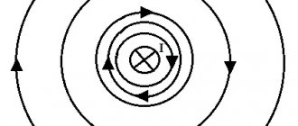
Magnetic induction of the ring
The induction of a straight wire has a small value and decreases with distance from the conductor, therefore it is practically not used in practical devices. The most widely used magnetic fields are those created by a wire wound around a frame. Therefore, such fields are called magnetic fields of circular current. The simplest such magnetic field is possessed by an electric current flowing through a conductor, which has the shape of a circle of radius R.
In this case, two cases are of practical interest: the magnetic field at the center of the circle and the magnetic field at point P, which lies on the axis of the circle. Let's consider the first case.
Magnetic induction at the center of a circular current.
In this case, each current element dl creates an elementary magnetic induction dB in the center of the circle, which is perpendicular to the contour plane, then the Biot-Savart-Laplace law will have the form
All that remains is to integrate the resulting expression over the entire length of the circle
where μ0 is the magnetic constant, μ0 = 4π•10-7 H/m,
I – current strength in the conductor,
R is the radius of the circle into which the conductor is rolled.
Let's consider the second case, when the point at which the magnetic induction is calculated lies on the straight line x , which is perpendicular to the plane limited by the circular current.
Magnetic induction at a point lying on the axis of a circle.
In this case, the induction at point P will be the sum of the elementary inductions dBX , which in turn is a projection onto the x- of the elementary induction dB
Applying the Biot-Savart-Laplace law, we calculate the value of magnetic induction
Now let’s integrate this expression over the entire length of the circle
where μ0 is the magnetic constant, μ0 = 4π•10-7 H/m,
I – current strength in the conductor,
R is the radius of the circle into which the conductor is rolled,
x is the distance from the point at which the magnetic induction is calculated to the center of the circle.
As can be seen from the formula for x = 0, the resulting expression transforms into the formula for magnetic induction at the center of the circular current.
Magnetic field of a circular current at its center
Figure 1. Magnetic field of a circular current at its center. Author24 - online exchange of student work
Let's consider a circular conductor through which a direct current $I$ flows (Fig. 1). Let us select the element $dl$ on this conductor, which can be considered rectilinear. If we move to another element of the same current, then to the third and so on, applying the rule of the right screw, then it is obvious that all the magnetic fields created by these elements in the center are directed along one straight line, perpendicular to the plane of the ring. This means, using the principle of superposition, we will replace vector addition with algebraic addition.
Let us write the Biot-Savart-Laplace law for the modulus of the field induction vector created by the element d$l_1$:
$dB=\frac{\mu_{0}\mu }{4\pi }\frac{Idl_{1}\sin \alpha }{r^{2}}\left( 5\right).$
From Fig. 1 we see:
- that the distance from the elementary current to the center of the turn is equal to its radius ($R$) and will be the same for all elements on this turn,
- the element $dl$ (like all other elements) will be normal to the radius vector $\vec r$.
Taking into account the said expression (5), we present it in the form:
$dB=\frac{\mu_{0}\mu }{4\pi }\frac{Idl_{1}}{R^{2}}\left( 6 \right)$.
Depersonalizing the turns with current, we further set $dl_1=dl$.
Since our current is continuous, to find the total field at its center, we integrate (6), we have:
$B=\oint\limits_L {dB=} \frac{\mu_{0}\mu }{4\pi}\frac{I}{R^{2}}\oint\limits_L {dl} =\frac{ \mu_{0}\mu }{4\pi}\frac{I}{R^{2}}2\pi R\to$
$B=\mu_{0}\mu \frac{I}{2R}\left( 7 \right)$.
Note 1
$L=2πR$ is the circumference of the coil.
Induction of the magnetic field of a circular current on its axis
Let's find the magnetic field induction on the axis of a circular current if the current flowing through it is equal to $I$, the radius of the turn is $R$ (Fig. 2).
Figure 2. Induction of the magnetic field of a circular current on its axis. Author24 - online exchange of student work
As a basis for accomplishing this task, we will take the Biot-Savart-Laplace law (1), where from Fig. 2 we see that:
- $\vec{r}=\vec{R}+\vec{h}$,
- $d\vec{l}\times \vec{r}=d\vec{l}\times \vec{R}+d\vec{l}\times \vec{h}(9).$
Using the superposition principle, law (1) for our current and formula (8-9) we write:
$\vec{B}=\oint\limits_L {dB=}$$\frac{\mu \mu_{0}}{4\pi }I\oint\limits_L \frac{d\vec{l}\times\ vec{r}}{r^{3}} $ $=\frac{\mu \mu_{0}}{4\pi }\frac{I}{r^{3}}\left( \oint\limits_L {d\vec{l}\times \vec{R}+} \oint\limits_L {d\vec{l}\times \vec{h}}\right)\left( 10 \right).$
In expression (10) when writing the integral, we took into account that the value of the vector $\vec{r}$ does not change. In addition, the vector $\vec h$, which determines the position of the point at which we are looking for the field, does not change when moving along our contour, therefore:
$\oint\limits_L {d\vec{l}\times \vec{h}} =(\oint\limits_L {d\vec{l})\times\vec{h}} =0\, \left( 11 \right),$
since ( $\oint\limits_L{d\vec{l})=0.}$
Let's calculate the integral: $\oint\limits_L {d\vec{l}\times \vec{R}.}$ Let's introduce a unit vector ($\vec n$), normal to the plane of the coil with the current.
$\oint\limits_L {d\vec{l}\times \vec{R}=\oint\limits_L {\vec{n}Rdl=\vec{n}R}} \oint\limits_L {dl=\vec{ n}R} 2\pi R=2\pi R^{2}\vec{n}\left( 12 \right)$.
We substitute the integration results from (12) into (10), we have:
$\vec{B}=\frac{\mu \mu_{0}}{4\pi }\frac{I}{r^{3}}2\pi R^{2}\vec{n}=\ frac{\mu\mu_{0}I}{2}\frac{R^{2}}{\left( R^{2}+h^{2}\right)^{\frac{3}{2 }}}\vec{n}\left( 13 \right)$
where, when recording the final result, we took into account that:
$r^{3}=\left( R^{2}+h^{2} \right)^{\frac{3}{2}}$.
Circulation of the magnetic induction vector
To calculate the magnetic induction of simple magnetic fields, the Biot-Savart-Laplace law is sufficient. However, with more complex magnetic fields, for example, the magnetic field of a solenoid or toroid, the number of calculations and the cumbersomeness of the formulas will increase significantly. To simplify calculations, the concept of circulation of the magnetic induction vector is introduced.
Circulation of the magnetic induction vector along an arbitrary contour.
's imagine some circuit l , which is perpendicular to the current I. At any point P of a given circuit, the magnetic induction B is directed tangentially to the given circuit. Then the product of vectors dl and B is described by the following expression
Since the angle dφ is quite small, the vector dlB is defined as the length of the arc
Thus, knowing the magnetic induction of a straight conductor at a given point, we can derive an expression for the circulation of the magnetic induction vector
Now it remains to integrate the resulting expression over the entire length of the contour
In our case, the magnetic induction vector circulates around one current, but in the case of several currents, the expression for the circulation of magnetic induction turns into the law of total current, which states:
The circulation of the magnetic induction vector in a closed loop is proportional to the algebraic sum of the currents that the given loop covers.
Magnetic flux. Gauss's theorem for magnetic field
The flow of the magnetic induction vector (or magnetic flux) through an arbitrary area S is characterized by the number of magnetic field lines penetrating a given area S.
If the area S is located perpendicular to the magnetic field lines (Fig. 14), then the flux FB of the induction vector through this area S:
.
Rice. 14 Fig. 15
If the area S is located non-perpendicular to the magnetic field lines (Fig. 15), then the flux ФB of the induction vector through this area S:
,
where α is the angle between the vectors and the normal to the area S.
,In order to find the flux FB of the magnetic induction vector through an arbitrary surface S, it is necessary to divide this surface into elementary areas dS (Fig. 16) and determine the elementary flux of the vector through each area dS using the formula:
where α is the angle between the vectors and the normal to a given area dS;
Then the vector flow through an arbitrary surface S is equal to the algebraic sum of elementary flows through all elementary areas dS into which the surface S is divided, which leads to integration:
– a vector equal in size to the area of the site dS and directed along the normal vector to the given site dS.
.
Gauss's theorem for magnetic field
For an arbitrary closed surface S (Fig. 17), the flux of the magnetic field induction vector through this surface S can be calculated using the formula:
.
On the other hand, the number of magnetic induction lines entering the volume bounded by this closed surface is equal to the number of lines emerging from this volume (Fig. 17). Therefore, taking into account the fact that the flux of the magnetic field induction vector is considered positive if the field lines exit the surface S, and negative for the lines entering the surface S, the total flux of the FB vector through an arbitrary closed surface S is equal to zero , i.e.:
,
which constitutes the formulation of Gauss's theorem for the magnetic field .
The phenomenon of electromagnetic induction. Faraday's law
The phenomenon of the occurrence of electric current in a closed conducting circuit as a result of a change in the magnetic flux penetrating this circuit is called the phenomenon of electromagnetic induction. The occurrence of an induced electric current in a circuit indicates the presence in this circuit of an electromotive force, called electromotive force (EMF) of electromagnetic induction.
According to Faraday's law, the magnitude of the electromagnetic induction emf is determined only by the rate of change of the magnetic flux passing through the conductive circuit, namely:
the magnitude of the EMF of electromagnetic induction is directly proportional to the rate of change of the magnetic flux penetrating the conducting circuit:
(Faraday's law).
The direction of the induced current in the circuit is determined by Lenz's rule : the induced current in the circuit always has such a direction that the magnetic field created by this current prevents the change in the magnetic flux that caused this induced current.
Faraday's law, taking into account Lenz's rule, can be formulated as follows: the magnitude of the EMF of electromagnetic induction in a circuit is numerically equal and opposite in sign to the rate of change of magnetic flux through the surface bounded by this circuit, that is:
(Faraday's law taking into account Lenz's rule).
To find the magnetic field induction in the center of a circular conductor with current, it is necessary to divide this conductor into elements, find a vector for each of them, and then add all these vectors. Since all vectors are directed along the normal to the plane of the coil (Fig. 11), the addition of vectors can be replaced by the addition of their modules dB.
According to the Biot-Savart-Laplace law, the vector modulus:
.
Since all elements of the conductor are perpendicular to the corresponding radius vectors, then sina = 1 for all elements. Distances r = R for all conductor elements. Then the expression for the modulus of the vector:
.
Now we can move on to integration:
.
So, the magnetic field induction in the center of a circular conductor with current is:
(R is the radius of the coil with current I).
The action of a magnetic field on a current-carrying conductor (Ampere’s law) and on a moving charge (Lorentz force)
Ampere's law. A conductor element with current I, placed in a magnetic field with induction (Fig. 12), is acted upon by a force ( – Ampere force ):
.
Vector module: ,
where is the angle between the vectors and .
The direction of the vector can be determined by the rule of the left hand: if the lines of force enter the palm, and four extended fingers are located along the current, then the abducted thumb will indicate the direction of the Ampere force vector.
(The force is perpendicular to the plane of Figure 12.)
Lorentz force . A charge q moving with speed in a magnetic field with induction (Fig. 13) is acted upon by a force ( – Lorentz force ):
.
Vector module: ,
where α is the angle between the vectors and .
The direction of the vector can be determined by the left hand rule for moving positive charges and by the right hand rule for moving negative charges:
if the magnetic field lines enter the palm, and the four extended fingers are located according to the speed of the particle, then the abducted thumb will indicate the direction of the Lorentz force (Fig. 13, the force is perpendicular to the plane of the figure).