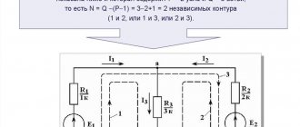
TOE › Magnetic circuits
A magnetic circuit is a device, individual sections of which are made of ferromagnetic materials through which the magnetic flux is closed. Examples of the simplest circuits are the magnetic circuits of the ring coil and the electromagnet shown in Fig. 6.11, a. Electrical machines and transformers, electromagnetic devices and devices usually have magnetic circuits of a more complex shape.
Rice. 6.11 Magnetic circuits (a - unbranched, b - branched)
If a magnetic circuit is made of the same material and has the same cross-section along its entire length, then the circuit is called homogeneous .
If individual sections of the chain are made of different ferromagnetic materials and have different lengths and cross-sections, then the chain is inhomogeneous .
Magnetic circuits, like electrical ones, can be branched (Fig. 6.11,6) and unbranched (Fig. 6.11,a).
In unbranched circuits, the magnetic flux Ф in all sections has the same value.
Branched chains can be symmetrical or asymmetrical . The circuit shown in Fig. 6.11.6, is considered symmetrical if its right and left parts have the same dimensions, are made of the same material and if the MMFs I1W1 and I2W2 are the same. If at least one of the specified conditions is not met, the circuit will be asymmetrical .
Let us divide an unbranched magnetic circuit, for example, in Fig. 6.11a, into a number of homogeneous sections, each of which is made of a specific material and has the same cross-section S along its entire length. The length of each section L will be considered equal to the length of the average magnetic line within this section. From the above it follows that the magnetic fluxes of all sections of an unbranched chain are equal, i.e.
Ф1=Ф2=Ф3=…=Фn,
and the field in each area can be considered homogeneous, i.e. Ф = BS; That's why
B1S1=B2S2=B3S3=…=BnSn
Where n is the number of chain sections. Magnetic voltage on any part of the magnetic circuit
Where H is Voltage (measured in amperes per meter A/M).
B - Magnetic induction (measured in Tesla).
L - Length of the average field line passing through the center of the cross section of the magnetic circuit.
S is the cross-sectional area of the magnetic circuit.
— Magnetic constant.
μr — Magnetic permeability of ferromagnets.
For a given direction of current in the winding, the direction of flow and MMF IW is determined by the gimlet rule.
9.1.1. Elements of a magnetic circuit
A magnetic circuit (magnetic circuit) is a collection of various ferromagnetic and non-ferromagnetic parts of electrical devices for creating magnetic fields of the desired configuration and intensity. Depending on the operating principle of the electrical device, the magnetic field can be excited either by a permanent magnet or by a current-carrying coil located in one or another part of the magnetic circuit.
The simplest magnetic circuits include a toroid made of homogeneous ferromagnetic material (Fig. 9.1). Such magnetic cores are used in multi-winding transformers, magnetic amplifiers, computer elements and other electrical devices.
In Fig. Figure 9.2 shows a more complex magnetic circuit of an electromechanical device, the moving part of which is drawn into an electromagnet by a direct (or alternating) current in the coil. The force of attraction depends on the position of the moving part of the magnetic circuit.
In Fig. Figure 9.3 shows a magnetic circuit in which the magnetic field is excited by a permanent magnet. If a moving coil located on a ferromagnetic cylinder is connected to a direct current circuit, then a torque acts on it. Rotating the current-carrying coil has virtually no effect on the magnetic field of the magnetic circuit. Such a magnetic circuit exists, for example, in measuring instruments of a magnetoelectric system.
The considered magnetic circuits, like other possible designs, can be divided into unbranched magnetic circuits (Fig. 9.1 and 9.3), in which the magnetic flux in any section of the circuit is the same, and branched magnetic circuits (Fig. 9.2), in which magnetic fluxes in different chain sections are different. In general, branched magnetic circuits can be of complex configuration, for example in electric motors, generators and other devices.
In most cases, a magnetic circuit should be considered nonlinear, and only under certain assumptions and certain operating conditions can a magnetic circuit be considered linear.
Practical use
Ohm's formula is often used to answer the following questions:
- Calculation of magnetomotive force.
- Calculation of the number of turns of wire that, at a given current, will provide the required amount of magnetic flux.
As an example, consider the magnetic circuit shown in the figure below.
Let's agree that the first section is made of cast steel, the second is made of electrical steel, and the third is an air gap. It is required to determine the number of turns of the winding capable of providing a magnetic flux, which is equal to 0.0036 Weber for a current of 2 Amperes. Based on the dimensions indicated in the diagram, you can calculate the lengths of sections and cross-sectional areas of the part:
To find the value of magnetic induction, the data from the conditions of the problem should be substituted into the appropriate formula.
To find the magnitude of the magnetic field strength, you will need to open a graph of the relationship between magnetic induction and intensity in the reference book and determine what value corresponds to 1.5 Tesla. For cast steel this value is approximately 700 A/m, and for electrical steel - 3000 A/m. For an air gap, the desired value can be obtained by using the appropriate formula:
Using Ohm's law for a magnetic circuit, you can determine the number of turns by substituting the found values:
Therefore, in the case under consideration, 4083.5 turns will be required to provide the required parameters.
As we can see, when solving practical problems in electrical engineering, it is convenient to use concepts such as magnetomotive force and magnetic resistance.
It should also be said that without magnetic fluxes there would probably not have been such an industry as electrical engineering. After all, the properties of the magnetic field are the basis for the operation of many modern devices, including transformers, electric motors, generators, measuring instruments, and various sensors.
9.1.2. Total current law for a magnetic circuit
The law of total current was obtained on the basis of numerous experiments. This law establishes that the integral of the magnetic field strength along any closed circuit (circulation of the intensity vector) is equal to the algebraic sum of the currents associated with this circuit:
(9.1)
Moreover, those currents whose direction corresponds to traversing the circuit in the direction of clockwise movement (gimlet rule) should be considered positive. In particular, for the contour in Fig. 9.4 according to the law of complete
current
Quantity S I
in (9.1) is called magnetomotive force (MF).
The basic SI unit of MMF is the ampere (A). The basic unit of magnetic field strength in the SI system—ampere per meter (A/m)—does not have a special name. A unit often used that is a multiple of the basic unit of magnetic field strength is ampere per centimeter, 1 A/cm = 100 A/m.
The magnetic circuit of most electrical devices can be represented as consisting of a set of sections, within each of which the magnetic field can be considered uniform, i.e., with a constant intensity equal to the magnetic field strength H k
along the midline of a section of length
lk
. For such magnetic circuits, integration in (9.1) can be replaced by summation.
If the magnetic field is excited by a coil with current I
, which has
w
turns, then for the contour of a magnetic circuit linked to the turns and consisting of
n
sections, instead of (9.1) we can write
(9.2 a),
If the circuit is connected to turns m
coils with currents, then
(9.2 b)
where Fp
= IpWp
- MMF.
Thus, according to the law of total current MMF F
equal to the sum of the products of the magnetic field strengths and the lengths of the corresponding sections for the magnetic circuit contour.
The product Hk · lk = U m k
is often called the magnetic voltage of a section of a magnetic circuit.
Magnetic reluctance and Ohm's law for a magnetic circuit.
By analogy with an electrical circuit, the value
is called the magnetic resistance of a section of a magnetic circuit ( measured in 1/H ).
Thus, the magnetic voltage
Expression (3), by analogy with an electric circuit, is often called
Ohm’s law for a magnetic circuit . However, due to the nonlinearity of the circuit caused by the variability of the magnetic permeability μr of ferromagnets, it is practically not used for calculating magnetic circuits.
9.1.3. Properties of ferromagnetic materials
The magnetic state of any point in an isotropic medium, i.e. a medium with identical properties in all directions, is completely determined by the magnetic field strength vector H
and the magnetic induction vector
B
, which coincide with each other in direction.
The basic unit of magnetic induction in the SI system is called tesla (T): 1 T = 1 Wb/m2 = 1 V s/m2. This is the induction of such a uniform magnetic field in which the magnetic flux Ф
through a surface of 1 m2 perpendicular to the direction of the magnetic field lines is equal to one Weber (Wb).
In a vacuum, induction and magnetic field strength are related by a simple relationship: B = m0H, where m 0 = 4p·10-7 H/m is the magnetic constant. For ferromagnetic materials, the dependence of induction on the magnetic field strength B ( H )
in the general case nonlinear.
In order to experimentally study the magnetic properties of a ferromagnetic material, it is necessary to carry out all measurements on a sample in which the magnetic field is uniform. Such a sample can be a toroid made of the ferromagnetic material under study (Fig. 9.5), the length of the magnetic lines in which is much greater than its transverse dimensions (thin-walled toroid). On the toroid there is a uniformly wound winding with the number of turns w
.
We can assume that in a toroid made of ferromagnetic isotropic material with tightly wound turns, all magnetic lines are circles, and the vectors of magnetic field strength and induction are directed tangentially to the corresponding circle. So, in Fig. 9.5 shows the average magnetic line and vectors H
and
B
at one of its points.
When calculating the strength and induction of the magnetic field in a thin-walled toroid, we can assume that all magnetic lines have the same length, equal to the length of the middle line 2 p
r
.
Let us assume that the ferromagnetic material of the thin-walled toroid is completely demagnetized and the current I
there is none in the winding (
B
= 0 and
H
= 0).
If we now smoothly increase the direct current I
in the coil winding, then a magnetic field will arise in the ferromagnetic material, the intensity of which is determined by the total current law (9.1):
H
= Iw /2 p r .
(9.3)
Each tension value H
The magnetic field in a thin-walled toroid corresponds to a certain magnetization of the ferromagnetic material, and, consequently, to the corresponding value of magnetic
induction B.
If the initial magnetic state of the material of a thin-walled toroid is characterized by the values of H
= 0,
B
= 0, then with a smooth increase in current we obtain a nonlinear dependence
B( H),
which is called the initial magnetization curve (Fig. 9.5, dashed line).
Starting from certain values of
the magnetic field
H B
in a thin-walled ferromagnetic toroid practically stops increasing and remains equal to
B max
.
This region of the B( H)
is called the technical saturation region.
If, having reached saturation, we begin to smoothly reduce the direct current in the winding, i.e., reduce the field strength (9.3), then the induction will also begin to decrease. However, the dependence B( H)
no longer coincides with the initial magnetization curve.
By changing the direction of the current in the winding and increasing its value, we obtain a new section of the dependence B( H).
At significant negative values of the magnetic field strength, technical saturation of the ferromagnetic material will occur again.
If we now continue the experiment: first reduce the reverse current, then increase the forward current until saturation, etc., then after several magnetization reversal cycles a symmetrical curve will be obtained for the B( H)
(Fig. 9.5, solid line).
This closed cycle B( H)
is called the limiting static hysteresis loop (or limiting static hysteresis cycle) of a ferromagnetic material.
If during symmetric magnetization reversal the technical saturation region is not reached, then the symmetric B( H)
is called a symmetric partial hysteresis loop of the ferromagnetic material.
The statistical limit cycle of hysteresis of ferromagnetic materials is characterized by the following parameters:
NS
- coercive force,
V r
- residual induction and
k = Br / BH - l 0 Hc
- squareness coefficient.
According to the value of the parameter H with
limiting static hysteresis cycle, ferromagnetic materials are divided into groups:
1) magnetic materials with low values of coercive force ( H s
< 0.05…0.01 A/m) are called soft magnetic;
2) magnetic materials with large values of coercive force ( H s
> 20…30 kA/m) are called hard magnetic.
Hard magnetic materials are used for the manufacture of permanent magnets, and soft magnetic materials are used for the manufacture of magnetic cores of electrical devices operating in magnetization reversal mode in extreme or frequent cycles.
Soft magnetic materials, in turn, are divided into three types: magnetic materials with a rectangular limiting static hysteresis loop, in which the rectangularity coefficient k
> 0.95 (Fig. 9.6, a);
magnetic materials with a rounded limiting static hysteresis loop, in which the squareness coefficient is 0.4 < < k
<0.7 (Fig. 9.6, b);
magnetic materials with linear properties, in which the dependence B ( H )
is almost linear:
B = m r m 0 N
(Fig. 9.6, c), where
m r
is the relative magnetic permeability.
All types of magnetic characteristics of ferromagnetic materials can be obtained from samples made either from various ferromagnetic alloys or from ferromagnetic ceramics (ferrites). A valuable property of ferrites, in contrast to ferromagnetic alloys, is their high electrical resistivity.
Magnetic cores made of ferromagnetic materials with a rectangular limiting static hysteresis cycle are used in the random access memory of digital computers, magnetic amplifiers and other automation devices. Ferromagnetic materials with a rounded limiting static hysteresis cycle are used in the manufacture of magnetic cores of electrical machines and devices. The magnetic cores of these devices usually operate in magnetization reversal mode in symmetrical private cycles. In basic calculations of the magnetic circuits of such electrical devices, symmetrical partial cycles are replaced by the main magnetization curve of the ferromagnetic material, which is the geometric locus of the vertices of the symmetrical partial cycles of a thin-walled ferromagnetic toroid (Fig. 9.7), obtained with a low-frequency sinusoidal current in the winding.
Using the main magnetization curve of a ferromagnetic material, the dependence of the absolute magnetic permeability is determined
m a
=
m r m 0
=
B/N
(9.4)
from tension N
magnetic field, which is shown in Fig. 9.7 with a dashed line.
In Fig. Figure 9.8 shows the main magnetization curves of some electrical steels used in electrical machines, transformers and other devices, as well as cast iron and permalloy.
Ferromagnetic materials with linear properties are used to make sections of magnetic circuits for inductors of oscillatory circuits with high quality factor. Such circuits are used in various radio devices (receivers, transmitters), in small-sized communication antennas, etc.
If on a section of a magnetic circuit with cross-sectional area S
Since the magnetic field is non-uniform, calculations can often be made using the average value of induction
Вср = Ф/ S
and the intensity
Нср
on the average magnetic line.
For example, for a toroid with a rectangular cross-section, internal radius rt ,
external radius
r 2
and height
h
, made of a magnetic material with linear properties
B = m r m 0 H
at
m r
= const (Fig. 9.6, c),
Where
From the obtained expressions it follows that
In the future, to simplify calculations, we will not take into account the inhomogeneity of the magnetic field in the cross section of each section of the magnetic circuit, and we will assume that the field in each section is uniform and is determined by the values of intensity and induction on the average magnetic line.
Lecture on UD "Electrical Engineering" on the topic: "Electromagnetism and magnetic induction"
Section 2. Electromagnetism and magnetic induction
Topic 1. Electromagnetism and magnetic induction
Target:
Introduction to the concept of a magnetic field, characteristics and parameters of a magnetic field. with a magnetic circuit. Study of Ohm's law and Kirchhoff's laws for a magnetic circuit, the law of electromagnetic induction, Lenz's principle. Determination of magnetic field energy. Calculation of magnetic circuits.
Tasks:
1. Familiarize yourself with the concept of a magnetic field, the characteristics and parameters of a magnetic field, and a magnetic circuit. Consider Ohm's law and Kirchhoff's laws for a magnetic circuit, the law of electromagnetic induction, Lenz's principle. Determine the energy of the magnetic field. Learn how to calculate magnetic circuits.
2. Improve the ability to apply basic terms and formulas in practice.
3. To promote an understanding of the essence and social significance of one’s future profession and the manifestation of a sustainable interest in it.
Information Support:
Main literature:
1. Sindeev Yu.G. Electrical engineering with the basics of electronics: A textbook for students of vocational schools and colleges. — Rostov-on-Don: Phoenix, 2014.
2. Turevsky I.S., Slavinsky A.K. Electrical engineering with fundamentals of electronics. Textbook for open source software. – M.: Forum, 2014.
Additional literature:
1. Danilov I.A. General electrical engineering with fundamentals of electronics. - M.: Higher School, 2012.
2. Ermuratsky P.V. Electrical and Electronics. – M.: DMK Press, 2011.
3. Kasatkin A.S. Basics of electrical engineering. – M.: Higher School, 2001.
Internet resources:
http:/antigtu.ru/video-lp/ - video lectures on electrical engineering; electronic lectures on electrical engineering; ready-made solutions to problems from various problem books.
Content
1.
The concept of a magnetic field.
2.
Characteristics and parameters of the magnetic field.
3.
Magnetic circuit.
4.
Ohm's law and Kirchhoff's laws for a magnetic circuit.
5.
Law of electromagnetic induction. Lenz's principle.
6.
Magnetic field energy.
7.
Calculation of magnetic circuits.
1.
Concept of magnetic field
Basic magnetic phenomena.
Since ancient times it has been known that some types of iron ore have the property of attracting iron. This ore was called a magnet.
A magnet exerts its influence not only on objects brought to it, but also on the space surrounding it. If we place small magnetic arrows around a linear magnet, we will see that they are positioned differently in relation to the magnet. Having removed the magnet, we see that all the arrows are set approximately in the north-south direction. Consequently, the presence of a magnet changes the properties of the space around it.
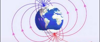
Figure 1. Location of magnetic field lines of a permanent magnet
The space in which the action of a magnet on a magnetic needle is detected is called a magnetic field, and the line along which the axis of the magnetic needle is established is called a magnetic line of force. It is generally accepted that the lines of force leave the north pole and enter the south.
Magnetic field of electric current.
Magnetic and electrical phenomena are closely related to each other. This can be easily verified by the following experiment. By installing a wire above the magnetic needle parallel to it and passing an electric current through it, we will notice that the needle will deviate from its previous position. But as soon as the current stops, the arrow returns to its original position.
From this experiment we can conclude that when current passes through a conductor, a magnetic field is formed around the latter: the magnetic needle is deflected by the current.
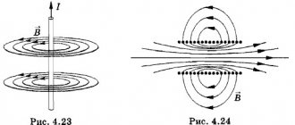
If several magnetic arrows are placed around a conductor through which an electric current passes, all the arrows will rotate and be positioned in the direction of the tangents to the circles: the magnetic field lines of a rectilinear current are closed concentric circles located in planes perpendicular to the direction of the current. When the direction of the current in the conductor changes, all the magnetic needles will turn and become in the opposite direction.
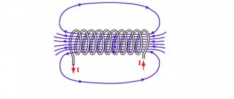
Solenoid
called a conductor twisted in a spiral through which an electric current is passed. If the solenoid is brought closer to the magnetic needle, we will see that one end of the solenoid attracts the south pole, and the other, the north pole. Consequently, the solenoid, when current passes through it, is similar in its magnetic properties to a straight magnet. The direction of the magnetic field lines and solenoid poles is determined using the "screw rule".
If a soft iron core is inserted inside the solenoid, and the solenoid is moved significantly away from the magnetic needle, the compass needle will still turn. This suggests that the iron core enhances the magnetic effect of the solenoid.
Electromagnet.
A solenoid with a steel core inside is called an electromagnet. Electromagnets are widely used in technology. With their help, magnetic fields are created in electric generators, electrical measuring instruments, relays, etc.
2.
Characteristics and parameters of the magnetic field
Magnetic permeability.
The ability of any material to be magnetized to one degree or another is determined by its magnetic permeability.
The magnetic permeability of ferromagnetic materials is different and exceeds the magnetic permeability of vacuum (magnetic constant). The number showing how many times the magnetic permeability of a ferromagnetic material is greater than the magnetic permeability of a vacuum is called relative magnetic permeability
.
By passing current through a coil with a core, we create a magnetic field. Consequently, the coil core becomes magnetized. The greater the current and the number of turns in the coil, the more the core is magnetized. This means that the magnitude of the magnetizing force is equal to the product of the current strength and the number of turns of the conductor in the coil.
Tension.
The magnetic field created by a conductor when current passes through it is characterized by intensity, which is determined by dividing the magnetizing force by the length of the coil and is designated
1 A/m
.
However, in practice, another unit of measurement is usually used, 80 times
larger than
1 A/m
, called
oersted
.
The intensity or strength of the field is assessed by the magnitude of the magnetic induction vector
. It is determined by the value of the force “F” created by the passing current “I” through a conductor of length “l”. В=F/(I∙l)
The SI unit of measurement of magnetic induction is Tesla (in memory of the physicist who studied these phenomena and described them using mathematical methods). In Russian technical literature it is designated “Tl”, and in international documentation the symbol “T” is adopted.
1 T is the induction of such a uniform magnetic flux, which acts with a force of 1 newton for each meter of length of a straight conductor perpendicular to the direction of the field, when a current of 1 ampere passes through this conductor.
1T=1∙N/(A∙m)
The direction of the vector is determined by the left-hand rule (Figure 2).
Figure 2. Rule
for determining the direction of the magnetic induction vector
If you position the palm of your left hand in a magnetic field so that the lines of force from the north pole enter the palm at right angles, and place four fingers in the direction of the current in the conductor, then the protruding thumb will indicate the direction of the force to this conductor.
The force acting on an electric current does not depend on the materials from which the conductor is made and its cross-sectional area. Even if this conductor does not exist at all, and moving charges begin to move in another medium between the magnetic poles, then this force will not change in any way.
If inside a magnetic field at all points the vector has the same direction and magnitude, then such a field is considered uniform.
Magnetic flux (F)
If we consider the passage of magnetic induction through a certain area S, then the induction limited by its limits will be called magnetic flux (Figure 3).
Figure 3. Illustration of determining the magnitude of magnetic flux
When the area is inclined at some angle α to the direction of magnetic induction, the magnetic flux decreases by the amount of the cosine of the angle of inclination of the area. Its maximum value is created when the area is perpendicular to its penetrating induction. Ф=В·S
The unit of measurement for magnetic flux is 1 weber, defined by the passage of induction of 1 tesla through an area of 1 square meter.
Electromagnetic induction.
We have already established that current produces a magnetic effect: the magnetic needle is deflected under the influence of the current passing through the conductor; an iron rod placed inside a current coil is magnetized; A conductor carrying current, being in a magnetic field, begins to move.
However, the opposite effect is possible. Under certain conditions, a magnetic field can excite an electric current. When a conductor moves in a magnetic field or the magnetic flux around it changes, an electromotive force ( emf
), under the influence of which an electric current is formed in a closed conductor. It was found that an electric current occurs in a conductor if the conductor and magnet move relative to each other. But induced current occurs in a conductor only if the conductor, during its movement, crosses magnetic lines of force. If a conductor moves along the lines of force without crossing them, no current arises in it. Induction current also occurs if the magnitude of the magnetic flux around the conductor changes.
The occurrence of an electric current in a closed conductor when it crosses magnetic lines of force is called electromagnetic induction, the resulting electromotive force ( emf
) is
inductive
, and the current is
inductive
.
Self-induction.
When an electrical circuit is closed and opened, a magnetic field is created and destroyed around the conductor.
A changing magnetic field crosses the conductor and creates an electromotive force of self-induction in it - emf.
self-induction . With any change in the “own” magnetic field of the conductor, it is intersected by the “own magnetic” lines and an emf appears in it. self-induction.
The inductance of an electrical circuit is measured in henries
(
Gn
).
A conductor has an inductance of 1 H
if, with a uniform change in the current in the conductor by
1 A
per
1 sec,
an emf is induced in it.
self-induction equal to 1
V.
Mutual induction.
Let's take two conductors, wind two coils out of them, place these coils at a certain distance from each other, and pass a varying current through one of the coils. Then the magnetic field created by this current will cross the turns of the second coil, in which an emf will arise. mutual induction, and therefore the electric current is mutually inductive. The current, in turn, will cause the appearance of a magnetic field, which will cross the turns of the first coil, also causing mutual induction emf in it. This process is called mutual induction.
3.
Magnetic circuit
Magnetic circuit
called a device in which a magnetic flux is closed. A magnetic circuit is a set of ferromagnetic and non-ferromagnetic parts of electrical devices necessary to create magnetic fields of the required configurations and intensity.
Depending on the operating principle of the electrical device, the magnetic field can be excited either by a permanent magnet or by a current-carrying coil located in one or another part of the magnetic circuit. Electromagnetic processes in a magnetic circuit are described using the following concepts: magnetomotive force (MF – F
), magnetic flux (F), magnetic voltage (
U
m), etc.
Magnetic circuits can be unbranched
, in which the magnetic flux in any section of the circuit is the same, and
branched
, in which the magnetic fluxes in different sections of the circuit are different.
Table 1. Schemes
of a branched and unbranched magnetic circuit
| Straight chain | Branched chain |
Branched magnetic circuits can be of complex configuration, for example in electric motors, generators and other devices.
Unbranched magnetic circuits are homogeneous
and
heterogeneous
Homogeneous
The magnetic circuit forms a closed magnetic circuit with a uniform magnetizing winding, and each turn of the winding creates lines of magnetic induction, which, closing along the magnetic circuit, merge into a common magnetic flux.
In such a circuit, magnetic lines pass in the same medium and the magnetic field strength along the lines does not change. As a rule, these are ring magnetic cores (toroids), which are used as standard samples used to determine the magnetic characteristics of materials.
Heterogeneous
a magnetic circuit is a magnetic circuit in which the magnetic circuit is not continuous, but, for example, with an air gap, therefore the magnetic flux and magnetic field strength in the ferromagnetic material and the air gap are different.
A magnetic circuit is a path along which a magnetic flux is closed. This path can pass entirely through the air.
| Figure 4. Examples of magnetic circuits |
Figure 4a shows a solenoid. The magnetic circuit here passes through the air. The magnetic resistance of air is very high, so even with a large magnetizing force, the magnetic flux is small.
To increase the magnetic flux, ferromagnetic materials (usually cast or electrical steel) that have lower magnetic resistance are introduced into the magnetic circuit.
In Figure 4, b
a straight electromagnet with an open core is presented. Magnetic lines travel only a small part of their path through the steel core, but most of their path they travel through the air. The poles of an electromagnet are determined using the “gimlet rule”.
The horseshoe-shaped electromagnet shown in Figure 4, in
, represents a magnetic circuit with better conditions for the passage of magnetic flux.
With this design, the flow passes most of the way through steel and a smaller part from the N
to the
S
through air.
In Figure 4, d
The design of a magnetic circuit used in electrical engineering and instrument making is presented. A steel armature is placed between the poles of the electromagnet. The magnetic lines pass most of their path along the steel and only a very small part (from a few fractions of a millimeter to 2–3 mm) pass through two air gaps.
4.
Ohm's law and Kirchhoff's laws for a magnetic circuit
Ohm's law :
magnetic voltage in any area
because..
If ,
where
is
the
magnetic
resistance . .
Magnetic flux is directly proportional to magnetic voltage and inversely proportional to magnetic resistance.
Kirchhoff's laws
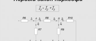
Kirchhoff's first law for magnetic circuits
states: the algebraic sum
of magnetic fluxes
in a node of a magnetic circuit is equal to zero.
Kirchhoff's first law is applied to the magnetic nodes of a branched magnetic circuit (Figure 5).
Figure 5. Magnetic flux distribution
Kirchhoff's second law for magnetic circuits
let's formulate as follows: the algebraic sum
of
magnetic stresses UM
=
H
l in a closed loop of a magnetic circuit (∑UM=∑H⋅l) is equal to the algebraic sum of
magnetomotive
forces F
=
I
w in the same loop (∑F=∑I⋅w) :
∑UM=∑F
or
∑H⋅l=∑I⋅w.
5.
The law of electromagnetic induction.
Lenz's rule In 1831, Faraday discovered one of the most fundamental phenomena in electrodynamics - the phenomenon of electromagnetic induction: in a closed conducting circuit, when the magnetic flux changes through a surface resting on this circuit, an electric current (induction current) arises.
It was found that the induced current always has such a direction that it prevents a change in the magnetic flux through a given conducting circuit. This pattern is called Lenz's rule
.
Figure 6. Illustration of Lenz's rule
In the case when we introduce a magnet into the coil (Figure 6), the magnetic flux in the circuit increases, which means that the magnetic field created by the induced current, according to Lenz’s rule, is directed against the increase in the magnet’s field. To determine the direction of the current, you need to look at the magnet from the north pole. From this position we will screw the gimlet in the direction of the magnetic field of the current, that is, towards the north pole. The current will move in the direction of rotation of the gimlet, that is, clockwise.
In the case when we remove the magnet from the coil, the magnetic flux in the circuit decreases, which means the magnetic field created by the induced current is directed against the decrease in the magnet's field. To determine the direction of the current, you need to unscrew the gimlet; the direction of rotation of the gimlet will indicate the direction of the current in the conductor - counterclockwise.
The appearance of an induced current means that when the magnetic flux changes in the circuit, an emf (induction emf) Ei
. Faraday established that the induced emf does not depend on the way in which the magnetic flux is changed: the area of the circuit changes, its orientation in the magnetic field changes, or the magnetic field penetrating the stationary circuit changes over time. In all cases, when the external magnetic flux penetrating the circuit changes, an induced current appears in the circuit. In this case, the value of the electromotive force is numerically equal to the rate of change of the magnetic flux, taken with the “-” sign.
where Ф is the magnetic flux through the circuit.
This formula expresses the law of electromagnetic induction
and “automatically” takes into account Lenz’s rule. When using formula (1), the direction of the normal to the surface bounded by the contour can be chosen arbitrarily, and the direction of traversing the contour must be related to the direction of the normal by the right screw rule. This determines both the sign of the magnetic flux and the “direction” of the induced emf in the circuit.
6.
Magnetic field energy
Magnetic field
shows how much work was spent by the electric current in the conductor (inductor) to create this magnetic field. Naturally, this energy will directly depend on the inductance of the conductor around which the magnetic field is created.
It turns out that the energy of the magnetic field is equal to half the product of the inductance of the circuit and the square of the current, i.e.
8.
Calculation of magnetic circuits
A magnetic circuit is similar to an electrical circuit. Magnetic flux F resembles electric current I, induction B resembles current density, magnetizing force (ns) Fm (H∙l=I∙ω) corresponds to e. d.s.
In the simplest case, the magnetic circuit has the same cross-section everywhere and is made of a homogeneous magnetic material. To determine the magnetizing force (n.s.) I∙ω necessary to ensure the required induction B, the corresponding strength H is determined from the magnetization curve and multiplied by the average length
of the magnetic field line l:
Fм =H∙l=I∙ω
.
From here the required current I or the number of turns ω of the coil is determined.
A complex magnetic circuit usually has sections with different cross-sections and magnetic materials. These sections are usually connected in series, so the same magnetic flux F passes through each of them. The induction B in each section depends on the cross section of the section and is calculated for each section separately using the formula B=Ф∶S.
For different values of induction, the voltage H is determined from the magnetization curve (Figure ?) and multiplied by the average length of the force line of the corresponding section of the circuit. By summing up the individual products, we get a complete n. With. magnetic circuit:
Fм=I∙ω=H1 ∙l1+H2 ∙l2+H3 ∙l3+…,
by which the magnetizing current or the number of turns of the coil is determined.
Figure 7. Magnetization curves
Examples
1. What should be the magnetizing current I of a coil having 200 turns in order for it to With. created a magnetic flux in a cast iron ring:
F = 15700 Mks = 0.000157 Wb?
The average radius of the cast iron ring is r=5 cm, and the diameter of its cross-section is d=2 cm (Figure 8).
Figure 8. Diagram of a closed magnetic circuit
Cross section of the magnetic circuit S=(π∙d2)/4=3.14 cm2.
The induction in the core is equal to: B=Ф∶S=15700∶3.14=5000 Gs.
In the MCSA system, the induction is equal to: B = 0.000157 Wb : 0.0000314 m2 = 0.5 T.
From the magnetization curve of cast iron we find for B = 5000 G = 0.5 T the required voltage H equal to 750 A/m. The magnetizing force is equal to: I∙ω=H∙l=235.5 Av.
Hence the required current I=(H∙l)/ω=235.5/200=1.17 A.
2. The closed magnetic circuit (Figure 9) is made of transformer steel plates. How many turns must a coil with a current of 0.5 A have in order to create a magnetic flux Ф = 160000 μs = 0.0016 Wb in the core?
Figure 9. Diagram of a closed magnetic circuit
Core cross section S=4∙4=16 cm2 =0.0016 m2.
Induction in the core B=Ф/S=160000/16=10000 Gs =1 T.
From the magnetization curve of transformer steel we find for B=10000 Gs =1 T the voltage H=3.25 A/cm =325 A/m.
Average length of magnetic field line l
=2∙(60+40)+2∙(100+40)=480=0.48 m.
Magnetizing force Fm=I∙ω=H∙l=3.25∙48=315∙0.48=156 Av.
At a current of 0.5 A, the number of turns is ω=156/0.5=312.
3. The magnetic circuit shown in Figure 10 is similar to the magnetic circuit in the previous example, except that it has an air gap of δ=5 mm. What should n be like? With. and the coil current so that the magnetic flux is the same as in the previous example, i.e. Ф = 160000 μs = 0.0016 Wb?
Figure 10. Diagram of an open magnetic circuit
The magnetic circuit has two series-connected sections, the cross-section of which is the same as in the previous example, i.e. S = 16 cm2. The induction is also equal to B = 10000 G = 1 T.
The average length of a magnetic line in steel is slightly shorter:
lс=48-0.5=47.5 cm ≈0.48 m.
Magnetic voltage on this section of the magnetic circuit
Hс ∙lс=3.25∙48≈156 Av.
The field strength in the air gap is:
Hδ=0.8∙B=0.8∙10000=8000 A/cm.
Magnetic voltage in the air gap section Hδ∙δ=8000∙0.5=4000 Av.
Full n. With. equal to the sum of magnetic stresses in individual areas: I∙ω=Hс ∙lс+Hδ∙δ=156+4000=4156 Av. I=(I∙ω)/ω=4156/312=13.3 A.
If in the previous example the required magnetic flux was provided by a current of 0.5 A, then for a magnetic circuit with an air gap of 0.5 cm, a current of 13 A is required to obtain the same magnetic flux. From this it can be seen that the air gap, even insignificant in relation to the length of the magnetic circuit, greatly increases the required n. With. and coil current.
Control questions
1. What is a magnetic field called?
2. What part of the field is the magnetic field?
3. What is magnetic induction called and how is it measured?
4. What does magnetic induction at a point depend on?
5. What determines the force of electromagnetic influence on a conductor?
6. What does the electromagnetic force of two current-carrying conductors depend on?
7. What is magnetic flux called and how is it measured?
8. What characterizes relative magnetic permeability?
9. What is magnetic field strength?
10. What is called electromagnetic induction?
11. What is the law of electromagnetic induction?
12. Formulate Lenz’s rule when an induced current occurs.
13. What is self-induced emf?
14. What is called the process of mutual induction?
9.1.4. Unbranched magnetic circuit
The task of calculating an unbranched magnetic circuit in most cases is to determine the MMF F
= Iw
, necessary in order to obtain the given values of magnetic flux or magnetic induction in a certain section of the magnetic circuit (most often in the air gap).
In Fig. 9.9 shows an example of an unbranched magnetic circuit - a magnetic circuit of constant cross-section S 1
with a gap.
The same figure shows other geometric dimensions of both sections of the magnetic circuit: the average length l 1
of the magnetic line of the first section made of ferromagnetic material and the length
l 2
of the second section - the air gap.
The magnetic properties of a ferromagnetic material are specified by the main magnetization curve B( H)
(Fig. 9.10) and thus, according to (9.4), by the dependence
m a (H).
According to the law of total current (9.2)
where H 1
and
H 2
- magnetic field strength in the first and second sections.
In the air gap, the values of magnetic induction B2
and tensions
H 2
are related by the simple relation
B2
=
m 0 H2
, and for a section of ferromagnetic material
B1
=
m a 1 H1.
In addition, in an unbranched magnetic circuit, the magnetic flux is the same in any cross section of the magnetic circuit:
Ф
= В1
S1 = B2S2 , ( 9.6 ) _
where S 1
and
S 2
- the cross-sectional area of the section of ferromagnetic material and the air gap.
If magnetic flux F
, then using (9.6) we find the values of the inductions
B 1
and
B 2
.
The field strength H 1
is determined from the main magnetization curve (Fig. 9.10), and
H 2
=
B 2
/
m 0
. Next, using (9.5), we calculate the required value of the MMF.
The inverse problem is more difficult: calculating the magnetic flux for a given MMF F
.
Replacing the magnetic field strengths in (9.5) with induction values, we obtain
,
or taking into account (9.6)
where rMk
= lk / Sk m ak
is the magnetic resistance
of the k
-th section of the magnetic circuit, and the magnetic resistance
the k
-th section is nonlinear if the dependence
B ( H )
for this section is nonlinear (Fig. 9.10), i.e.
m ak
≠ const.
For a section of a circuit with nonlinear magnetic resistance rM
it is possible to construct a Weber-ampere characteristic - the dependence of the magnetic flux
Ф
on the magnetic voltage
UM
in this section of the magnetic circuit.
The Weber-ampere characteristic of a section of the magnetic circuit is calculated from the main magnetization curve of the ferromagnetic material B ( H )
.
To construct the Weber-ampere characteristic, you need to multiply the ordinates and abscissas of all points of the main magnetization curve, respectively, by the cross-sectional area of the section S
and its average length
l
.
In Fig. 9.11 shows the Weber-ampere characteristics F
(
UM 1
) for a ferromagnetic section with nonlinear magnetic resistance
rM 1
and
Ф
(
UM
2) for an air gap with constant magnetic resistance
rM
2 =
l 2 / S 2 m 0
of the magnetic circuit according to Fig. 9.9.
It is easy to establish an analogy between the calculations of nonlinear DC electrical circuits and magnetic circuits with constant MMF. Indeed, from equation (27.7) it follows that the magnetic voltage on a section of the magnetic circuit is equal to the product of the magnetic resistance of the section and the magnetic flux UM
=
rM F
.
This dependence is similar to Ohm's law for a resistive element of a direct current electrical circuit U = rI
.
The sum of magnetic voltages in the circuit of a magnetic circuit is equal to the sum of the MMF of this circuit S UM
=
S F
, which is similar to Kirchhoff’s second law for direct current electrical circuits
S U
=
S E .
Continuing further the analogy between direct current electrical circuits and magnetic circuits with constant MMF, let us imagine an unbranched magnetic circuit (Fig. 9.9) with an equivalent circuit (Fig. 9.12, a).
As an illustration, we will limit ourselves to the use of graphical methods for the analysis of an unbranched magnetic circuit: the method of adding Weber-ampere characteristics (Fig. 9.11) and the load characteristic method (Fig. 9.12, b).
According to the first method, we will construct the Weber-ampere characteristic of the entire unbranched magnetic circuit Ф
(
UM 1
+
UM
2), graphically adding the Weber-amp voltage characteristics of its two sections.
With a known MMF F = Iw
A
from the Weber-ampere characteristic of the entire magnetic circuit , i.e., the magnetic flux
Ф
, and from the Weber-ampere characteristics of sections of the magnetic circuit - the magnetic voltages on each of them.
According to the second method, for the second (linear) section we will construct a load characteristic
i.e., a straight line passing through point F
on the abscissa axis and the point
F
/
rM 2
on the ordinate axis.
The intersection point A
of the load characteristic with the Weber-ampere characteristic of the ferromagnetic section of the circuit Ф(
UM 1
) determines the magnetic flux
Ф
in the circuit and the magnetic voltages on the ferromagnetic section
UM 1
and the air gap
UM 2
.
The induction value in the air gap is B 2 = Ф/ S 2
.
Basic parameters of magnetic circuits
From a physics course we know that any current-carrying conductor induces a magnetic field around itself. Thus, a magnetic field arises in the space surrounding moving electric charges and permanent magnets.
In matter, the magnetic field is excited not only by electric currents flowing through wires, but also by the movement of charged particles inside the atoms and molecules themselves.
The magnetic field in a substance can be microscopic and macroscopic. A microscopic field is a true field excited by moving elementary charges of matter. It changes dramatically over atomic-scale distances. The macroscopic field is obtained from the microscopic one by smoothing, that is, averaging over physically infinitesimal volumes of space.
The magnetic field is clearly depicted by magnetic lines of force, which determine the direction of the magnetic field in space. These lines have neither beginning nor end, that is, they are closed.
In the space surrounding the magnet, the positive direction of the field lines is taken to be the direction from the north pole to the south. The stronger the magnetic field, the higher the density of field lines. The magnetic field can be determined using a magnetic needle, which at each point in the field is set tangent to the magnetic field line.
The magnetic field lines of a straight conductor carrying current have the form of concentric circles (Fig. 16.1).
Magnetomotive force (MMF)
Main article: Magnetomotive force
Just as electromotive force (EMF) controls the flow of electric charge in electrical circuits, magnetomotive force (MMF) “controls” magnetic flux through magnetic circuits. The term magnetomotive force, however, is a misnomer because it is not a force or anything that moves. Perhaps it's better to just call it MMF. By analogy with the definition of EMF, the magnetomotive force F { Displaystyle { mathcal {F} }} around a closed loop is defined as:
F = ∮ HOUR ⋅ d l . { displaystyle { mathcal {F} } = oint mathbf {H} cdot mathrm {d} mathbf {l}.}
MMF represents the potential that a hypothetical magnetic charge would gain by completing a cycle. Controlled magnetic flux is no
magnetic charge current; it simply bears the same relation to MMF as electric current has to EMF. (See detailed description of microscopic sources of resistance below.)
The unit of magnetomotive force is the ampere-turn (At), represented by a steady direct electric current of one ampere flowing in a single-turn loop of electrically conductive material into a vacuum. Gilbert (Gb), established by IEC in 1930[1] This is the CGS unit of magnetomotive force and is a unit slightly smaller than the ampere-turn. The apartment is named after William Gilbert (1544–1603), an English physician and natural philosopher.
1 GB = 10 4 π V ≈ 0.795775 V { displaystyle { begin {align} 1 ; { text {Gb}} & = { frac {10} {4 pi}} ; { text {At}} & approximately 0.795775 ; { text {At}} end {align}}} [2]
Magnetomotive force can often be quickly calculated using Ampere's Law. For example, the magnetomotive force F { Displaystyle { mathcal {F} }} of a long coil is:
F = N i { displaystyle { mathcal {F} } = NI}
where N
this is the number of turns and
I
is the current in the coil.
In practice, this equation is used for the MMF of real inductors with N
being the winding number of the induction coil.