Kirchhoff's law (Kirchhoff's rules), formulated by Gustav Kirchhoff in 1845, are consequences of the fundamental laws of charge conservation and irrotational electrostatic field.
Kirchhoff's law is the relationship between currents and voltages in sections of any electrical circuits. They allow you to calculate any electrical circuit: direct, alternating or quasi-stationary current.
When formulating Kirchhoff's rules, concepts such as branch, circuit and node of an electrical circuit are used.
- Branch – a section of an electrical circuit with the same current.
- A node is a point at which three or more branches connect.
- A circuit is a closed path passing through several nodes and branches of a branched electrical circuit.
When traversing, it is necessary to take into account that a branch and a node can simultaneously belong to several circuits. Kirchhoff's rules are valid for both linear and nonlinear circuits for any type of change in currents and voltages over time. Kirchhoff's rules are widely used in solving electrical engineering problems due to their ease of calculation.
Examples of circuit calculations
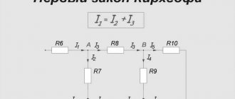
Let's look again at Figure 3. It shows 4 multidirectional vectors: i1, i2, i3, i4. Of these, two are incoming (i2, i3) and two are outgoing from the node (i1, i4). We will consider as positive those vectors that are directed to the point of connection of the branches, and the rest as negative.
Then, using the Kirchhoff formula, we will compose an equation and write it in the following form: – i1 + i2 + i3 – i4 = 0.
In practice, such nodes are part of contours, bypassing which you can create several more linear equations with the same unknowns. The number of equations is always sufficient to solve the problem.
Let's consider the solution algorithm using the example of Fig. 5.
Rice. 5. Calculation example
The circuit contains 3 branches and two nodes, which form three pairs of two independent circuits:
- 1 and 2.
- 1 and 3.
- 2 and 3.
Let us write an independent equation that is satisfied, for example, at point a. From Kirchhoff’s first rule it follows: I1 + I2 – I3 = 0.
Let's use Kirchhoff's second rule. To compose equations, you can select any of the contours, but we need contours with node a, since we have already compiled an equation for it. These will be circuits 1 and 2.
We write the equations:
We solve the system of equations:
Since the values of R and E are known (see Figure 5), we arrive at a system of equations:
Solving this system, we get:
- I1 = 1.36 (values in milliamps).
- I2 = 2.19 mA;
- I3 = 3.55 mA.
The potential of node a is equal to: Ua = I3*R3 = 3.55 × 3 = 10.65 V. To ensure that our calculations are correct, let’s check the fulfillment of the second rule in relation to circuit 3:
E1 – E2 + I1R1+ I2R2 = 12 – 15 + 1.36 – 4.38 = – 0.02 ≈ 0 (taking into account errors associated with rounding numbers during calculations).
If the verification of the implementation of the second rule is successfully completed, then the calculations were made correctly and the data obtained are reliable.
By applying Kirchhoff's rules (laws), it is possible to calculate the parameters of electrical energy for magnetic circuits.
Source
Formulation of the rules
Each Kirchhoff rule has universal properties. Both the first and second, although they do not relate to fundamental laws, are firmly substantiated.
Definitions
Before considering the simple principles and meaning of solving CS (systems of equations), you need to decide on the formulations used. In the typology of chains, the following concepts are used:
- branch;
- node;
- circuit.
All these are elements of an electrical circuit (EC).
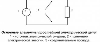
Elements of EC
The part of an electrical circuit through which electricity of the same magnitude passes is called a branch. The place where three or more branches connect is called a node. Typically, on diagrams, nodes are indicated by large dots. A circuit is the path along which electric current flows, passing through several sections of the EC, including nodes and branches.
Important! Current (I), leaving one point in the circuit and once passing through branches and nodes, must necessarily return to the beginning. A circuit is a closed circuit
Nodes and branches that are subject to the contour being studied at a certain moment can be part of other contours: they are common to several closed ECs at the same time.
First rule
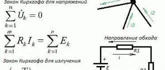
Kirchhoff's first law sounds like this: “The sum of all currents in the EC nodes is equal to zero.” If you give direction to the currents flowing through the intersections of conductors that have a common contact (node), then you can mark the inflowing currents with arrows pointing to the node. It is convenient to mark the flowing currents with arrows directed away from the node:
I1 + I2 – I3 – I4 – I5 = 0
Picture of the direction of movement of electricity
Conventionally assuming that incoming I have a positive sign, and outgoing ones have a negative sign, we can rephrase the statement. According to the law of conservation of charge, the algebraic sums of I entering and leaving a node are equal in value.
First Law
You can verify the truth of the first rule by assembling a mixed circuit for connecting resistors as a load for a power source U = 3 V.
Ammeters included in the branches allow you to visually record the values of currents entering and leaving the first node. Their algebraic sum (taking into account the signs) will be equal to zero.
Circuit diagram with installation of ammeters
Demonstration of Kirchhoff's voltage law in a parallel circuit
Kirchhoff's voltage rule (Kirchhoff's second law) will work for any circuit configuration at all, not just simple series circuits
Notice how this works for the following parallel circuit:. Figure 7 – Parallel circuit of resistors
Figure 7 – Parallel circuit of resistors
In a parallel circuit, the voltage across each resistor is equal to the supply voltage: 6 volts. Summing up the voltages along the 2-3-4-5-6-7-2 circuit, we get:
\
Please note that I designated the final (total) voltage as E2-2. Since we started our step-by-step path along the contour at point 2 and ended at point 2, the algebraic sum of these voltages will be the same as the voltage measured between the same point (E2-2), which of course must be zero
Problem 2
Knowing the resistance of the resistors and the emf of three sources, find the emf of the fourth and the currents in the branches.
As in the previous problem, we begin the solution by composing equations based on Kirchhoff’s first law. Number of equations n-1= 2
Then we compose equations according to the second law for three circuits. We take into account the directions of the traversal, as in the previous problem.
Based on these equations, we create a system with 5 unknowns
Having solved this system in any convenient way, we find the unknown quantities
For this task, we will perform a check using a power balance, in which the sum of powers given by the sources must be equal to the sum of the powers received by the receivers.
The power balance has converged, which means the currents and EMF are found correctly.
After reading articles about Kirchhoff’s first and second laws, a dear reader may say: “Okay, MyElectronix, you told me, of course, interesting things, but what should I do next with them? So far, based on your words, I have concluded that if I put together a diagram with my own hands, then I will be able to measure these dependencies in each of its nodes and in each circuit. That's great, but I'd like to calculate patterns rather than just observe dependencies!”
Gentlemen, all these comments are absolutely correct and in response to them we can only talk about the calculation of electrical circuits using Kirchhoff’s laws. Without further ado, let's get straight to the point!
Let's start with the simplest case. It is shown in Figure 1. Let's say the EMF of the power source is E1=5 V, and the resistances R1=100 Ohm, R2=510 Ohm, R3=10 kOhm. It is required to calculate the voltage across the resistors and the current through each resistor.
Gentlemen, I will note right away that this problem can be solved in a much simpler way than using Kirchhoff’s laws. However, now our task is not to look for optimal solutions, but to use a clear example to consider the methodology for applying Kirchhoff’s laws when calculating circuits.
Figure 1 – Simple diagram
In this diagram we can see three circuits. If the question arises – why three, then I recommend looking at the article about Kirchhoff’s second law. In that article there is almost the same diagram with a visual explanation of the method for calculating the number of circuits.
Gentlemen, I want to point out one subtle point. Although there are three circuits, there are only two independent ones. The third circuit includes all the others and cannot be considered independent. And in general, in all calculations we should always use only independent contours. Don't be tempted to write another equation at the expense of this general outline, nothing good will come of it.
So, we will use two independent circuits. To do this, we specify in each contour the direction of traversal of the contour. As we have already said, this is a certain direction in the circuit, which we take as positive. To some extent, we can call this an analogue of coordinate axes in mathematics. We will draw the direction of traversal of each contour with a blue arrow.
Next, let's set the direction of the currents in the branches: we'll just put it at random. It doesn’t matter whether we guess the direction now or not. If you guessed right, then at the end of the calculation we will receive a current with a plus sign, and if we were wrong, with a minus sign. So, let's denote the currents in the branches with black arrows labeled I1, I2, I3.
Kirchhoff's law for a magnetic circuit
The use of independent equations is also possible when calculating magnetic circuits. The Kirchhoff rules formulated above are also valid for calculating the parameters of magnetic fluxes and magnetizing forces.
Rice. 4. Magnetic circuits
In particular: ∑Ф=0.
That is, for magnetic fluxes, Kirchhoff’s first rule can be expressed in the words: “The algebraic sum of all possible magnetic fluxes relative to a node of a magnetic circuit is equal to zero.
Let us formulate the second rule for magnetizing forces F: “In a closed magnetic circuit, the algebraic sum of magnetizing forces is equal to the sum of magnetic stresses.” This statement is expressed by the formula: ∑F=∑U or ∑Iω = ∑НL, where ω is the number of turns, H is the magnetic field strength, and the symbol L denotes the length of the center line of the magnetic circuit. (It is conventionally assumed that each point of this line coincides with the lines of magnetic induction).
The second rule used to calculate magnetic circuits is nothing more than an alternative form of representing the total current law.
When the magnetic flux vectors coincide with the bypass directions (in some sections), we take the voltage drop on these branches with the “+” sign, and those counter to it with the “–” sign.