- Equations and graphs
- Rationale for vector diagram
- Effective value of alternating current
Sinusoidal emf. and current:
The receipt, transmission and use of electrical energy is carried out mainly using alternating current devices and structures. For this purpose, generators, transformers, transmission lines and AC distribution networks are used. The most widely used electrical energy receivers are those operating on alternating current. Alternating electric current is an electric current that changes over time (see Fig. 2.1, curves 2, 3).
A periodic electric current that is a sinusoidal function of time is called a sinusoidal electric current.
In practice, this current is usually meant when talking about alternating current. In some cases, the current varies according to a periodic non-sinusoidal law.
In linear electrical circuits, alternating sinusoidal current arises under the influence of e. d.s. the same shape. Therefore, to study electrical devices and alternating current circuits, it is necessary to first consider methods for obtaining sinusoidal e. d.s. and basic concepts related to quantities that vary sinusoidally.
Obtaining sinusoidal emf.
To get e. d.s. An industrial-type sinusoidal alternating current generator has certain design features. However, the fundamentally sinusoidal dependence of e. d.s. versus time can be obtained by rotating a conductor in the form of a rectangular frame at a constant frequency in a uniform magnetic field (Fig. 12.1).
Rice. 12.1. Rectangular frame in a magnetic field
Rotation of a coil in a uniform magnetic field
According to formula (10.5), e. d.s. in a frame having two active conductors of length l,
With uniform rotation of the frame, the linear speed of the conductor does not change: and the angle between the direction of the speed and the direction of the magnetic field changes in proportion to time: Angle β determines the position of the rotating frame relative to the plane perpendicular to the direction of magnetic induction. (The position of the frame at the start of time t = 0 is characterized by the angle β = 0.) Therefore, e. d.s. in the box is a sinusoidal function of time. The greatest value of e. d.s. reaches at angle In the case considered, the sinusoidal change in e. d.s. is achieved by continuously changing the angle at which the conductors intersect the lines of magnetic induction. However, this method of obtaining e. d.s. is not used in practice, since it is difficult to create a uniform field in a sufficiently large volume.
Alternator
In electric machine alternating current generators of industrial type, sinusoidal e. d.s. obtained at a constant angle, but in a non-uniform magnetic field.
The magnetic field of the generator (radial) in the air gap between the stator and the rotor is directed along the radii of the rotor circle (Fig. 12.2, a). Magnetic induction along the air gap is distributed according to a law close to sinusoidal. This distribution is achieved by the appropriate shape of the pole pieces. The sinusoidal distribution law of magnetic induction along the air gap is shown in Fig. 12.2, b in expanded form.
Rice. 12.2. Alternator circuit diagram. Distribution of magnetic induction along the air gap
Rice. 12.3. Circuit diagram of an alternator with two pairs of poles on the rotor
Rice. 12.4. Generator circuit with three turns (windings)
At any point in the air gap, the position of which is determined by the angle β measured from the neutral plane (neutral) counterclockwise, the magnetic induction is expressed by the equation
The neutral plane is perpendicular to the axis of the poles and divides the magnetic system into symmetrical parts, one of which belongs to the north pole, and the other to the south.
The magnetic induction has the greatest value under the middle of the poles, i.e. at angles and At the neutral (at β = 0 and β = 180°), the magnetic induction is zero (B = 0). In Fig. Figure 12.3 shows the design diagram of an alternating current generator with two pairs of poles located on the rotor, and the conductors of the winding where the electricity is induced. d.s., placed in the grooves of the stator core.
Let us note another type of alternating current generators - a generator with three windings (three-phase generator), which in the diagram in Fig. 12.4 are represented by three turns on the rotor (for turbogenerators and hydrogenerators, these windings are located on the stator). The planes of the turns are at an angle of 120° to each other.
E.D.S. in the generator winding
With uniform rotation of the rotor in its winding (in Fig. 12.2, a - in a coil), e.m. is induced. d.s., determined by formula (10.4). Substituting the expression for magnetic induction (12.3), we obtain
At β = 90°, i.e. in the position of the conductor under the middle of the pole, the greatest e is induced. d.s. Equation e. d.s. can be written as follows: Taking into account formula (12.1), we obtain the same dependence of the emf. from time, as when rotating the frame (see Fig. 12.1), considering the initial position of the coil (t = 0), when its plane coincides with the neutral: Thus, in this case, e. d.s. is a sinusoidal function of time (Fig. 12.5). The same result is obtained if the poles are rotated and the conductors are left motionless.
Rice. 12.5. Graph of sinusoidal e. d.s.
In a rectangular coordinate system, e. d.s. can be represented as a function of angle or as a function of time t. The dependence and can be depicted by one curve, but with different scales along the abscissa axis, differing by ω times. If the generator winding is closed through a resistance, then a sinusoidal current appears in the resulting circuit, repeating the shape of the e curve. d.s. Assuming the circuit resistance to be linear, equal to R, we obtain the following expression for the current: where is the largest current value. Sinusoidal voltage and current can be obtained using generators that do not have rotating parts and magnetic poles, such as tube generators.
Problem 12.1.
E.m.f. electric machine generator is expressed by the equation. Determine the number of pole pairs of this generator if the rotor speed n = 75 rpm is known. At what angle in space does the generator rotor rotate during 1/4 of a period? Solution. Period e. d.s., induced in the winding of a generator (see Fig. 12.2), which has one pair of poles, is equal to the time of full rotation of the rotor. The angular speed of rotation of the rotor can be determined by the ratio of the total angle corresponding to one revolution of the rotor to the period: However, the generator may have not one, but p pairs of poles (in Fig. 12.3 p = 2). Full cycle of change e. d.s. in this case, it occurs when the conductor moves past one pair of poles (as during a full revolution of the rotor in a generator with p = 1), therefore, at the same rotor speed, the emf period With. will be p times shorter, and the frequency will be p times greater. A decrease in period and a corresponding increase in frequency for a given number of pole pairs can be obtained by increasing the rotor speed. Frequency of sinusoidal e. d.s. at p = 1 it is equal to the number of rotor revolutions per second, and at p > 1 where n is the rotor speed, rpm. From Eq. d.s. the angular frequency ω = 314 rad/s is known; while at rotor speed n = 75 rpm
At p = 1, in 1/4 of the period the rotor will rotate 1/4 of the circle, i.e., angularly by 90º. At p = 40, the angle of rotation of the rotor for 1/4 of the period will be p times less:
Equations and graphs of sinusoidal quantities
It is impossible to analyze AC electrical circuits without expressing e. d.s. currents, voltages and their equations. For clarity, graphs of these quantities in a rectangular coordinate system are used. Therefore, let's look at the equations and graphs of sinusoidal quantities in more detail.
Equations and graphs
Equation (12.4) is written for the case when the beginning of the time count (t = 0) coincides with the moment the coil passes through the neutral (in Fig. 12.2, a is position 1, in which the plane of the coil coincides with the neutral).
In Fig. 12.4, the position of the turns also corresponds to the beginning of the time count (t = 0) and is determined for each of them by an angle measured from the neutral to the plane of the turn: for the first turn, this angle for the second - and third - When the rotor rotates, e. d.s. will be induced in all turns, but the emf equations will not be the same. Indeed, at = 0 e. d.s. in turns: This dependence e. d.s. from the initial position of the coil is taken into account by introducing the initial angle into the equation. Taking into account the initial angle e. d.s. turn C is expressed by the equation
e. d.s. turn B
Thus, in general form, the equation e. d.s. should be written like this:
From this equation you can determine the value of e. d.s. at any moment at an arbitrary initial position of the coil. In Fig. 12.6, in accordance with equation (12.6), graphs of the emf of three turns are plotted, differing at the start of the time count by their location relative to the neutral plane (eA at eC at eB at ).
Rice. 12.6. Graphs e. d.s., phase shifted
Characteristics of sinusoidal quantities
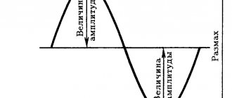
The equation and graph specify all the characteristics of a sinusoidally varying quantity: amplitude, angular frequency, initial phase, period, frequency, and instantaneous value for any moment in time.
The following are definitions of these characteristics and they are shown in Fig. 12.7 in relation to sinusoidal e. d.s. The definitions apply to all quantities that vary according to a sinusoidal law (current, voltage, etc.).
Rice. 12.7. On the question of the characteristics of periodic e. d.s.
Instantaneous value (or instantaneous value) e. d.s. e is the value of e. d.s. at the moment in time under consideration. Instant e. d.s. is determined by equation (12.6) by substituting into it the time t that has passed from the beginning of the countdown to a given moment.
Period T is the shortest time interval after which the instantaneous values of the periodic e. d.s.. are repeated. If the argument of the sine function is expressed in angles, then the period is expressed by the constant value 2π. Frequency f is the reciprocal of the period: that is, the frequency is equal to the number of periods of the variable e. d.s. per second. Frequency is expressed in hertz (Hz): 1 Hz = 1/s. Amplitude Em is the largest value that e takes. d.s. during the period. Amplitude is one of the instantaneous quantities that corresponds to an argument equal to , where k is any integer or zero. Phase (phase angle) is the argument of the sinusoidal emf, measured from the nearest previous e.m. transition point. d.s. through zero to a positive value. The phase at any time determines the stage of the harmonic change of the sinusoidal e. d.s. The initial phase ψ is the phase of the sinusoidal emf. at the initial moment of time. Two sinusoidal quantities having different initial phases are said to be out of phase. Angular frequency ω is the rate of phase change. During one period T, the phase angle uniformly changes by 2π, therefore
Problem 12.4.
Alternating electric current is given by the equation
Determine the period, frequency of this current and its instantaneous values at t = 0; t1 = 0.152 s. Draw a current graph. Solution. The sinusoidal current equation in the general case has the form Comparing this equation with the given partial current equation, we establish that the amplitude Im = 100 A, angular frequency ω = 628 rad/s, initial phase ψ = -60°. Period Frequency
Rice. 12.8. For Problem 12.4
We find the instantaneous current values by substituting the given time values into the current equation:
at t = 0 at t1 = 0.152 s The sinusoidal value is repeated after 360°, so the instantaneous current at the angle will be the same as at the angle: To construct a graph, you need to determine a series of instantaneous currents corresponding to different moments of time (Fig. 12.8).
Vector diagrams
Until now, quantities varying according to a sinusoidal law were specified by equations and depicted by graphs in a rectangular coordinate system. When calculating AC electrical circuits, they use a very simple and visual method of graphically representing sinusoidal quantities using rotating vectors.
Rationale for vector diagram
Let us assume that the current is given by the equation Let us draw two mutually perpendicular axes and from the point of intersection of the axes we draw the vector Im, the length of which on a certain scale Mi expresses the amplitude of the current Im:
Rice. 12.10. On the issue of vector diagram
We choose the direction of the vector so that with the positive direction of the horizontal axis the vector makes an angle equal to the initial phase ψ (Fig. 12.10).
The projection of this vector onto the vertical axis determines the instantaneous current at the initial moment of time: Let us imagine that the vector Im rotates counterclockwise with an angular velocity equal to the angular frequency ω. Its position at any moment of time is determined by the angle. Then the instantaneous current for an arbitrary moment of time t can be determined by the projection of the vector Im onto the vertical axis at this moment in time. For example, for t = t1 in the general case, we obtained the same equation as the alternating current was specified, which indicates the possibility of depicting the current as a rotating vector when applied to the drawing: in the initial position.
Construction of a vector diagram
By rotating the vector Im' counterclockwise, in a rectangular coordinate system we will construct a graph of changes in its projection onto the vertical axis within one revolution (one period). We obtain the already known graph of the sinusoidal function corresponding to the given equation.
When constructing vectors, positive angles are counted from the positive direction of the horizontal axis counterclockwise, and negative angles are counted along its movement.
In the process of calculating an electrical circuit, a number of sinusoidal quantities are determined. All of them can be depicted on one drawing using rotating vectors, tied to one pair of mutually perpendicular axes.
A set of vectors depicting in one drawing several sinusoidal quantities of the same frequency at the initial moment of time is called a vector diagram. For example, voltage and current in an electrical circuit are expressed by the equations
The vector diagram of such a circuit is shown in Fig. 12.11. If you choose the voltage and current scales then
Rice. 12.11. Vector diagram of current and voltage
A vector diagram contains vectors of sinusoidal quantities of the same frequency, so they rotate with the same frequency and their relative positions do not change.
The time reference point is chosen arbitrarily, so one of the diagram vectors can be directed arbitrarily; the rest must be positioned taking into account the phase shift relative to the first or previous vector.
Addition and subtraction of vectors
The simplicity and clarity of vector diagrams is not the only and not the main advantage of the method of depicting sinusoidal quantities. It is required to add, for example, two currents given by equations. The expression for the sum turns out to be cumbersome, and the amplitude and initial phase of the resulting current are not visible from it.
You can graphically add two given currents, plotting them in one coordinate system and for a number of arguments, finding the sum of two ordinates. We draw a sum curve through the obtained points and see that this curve is also a sinusoid with the same period as the terms. From the total current curve you can find the amplitude and initial phase. The bulkiness and inconvenience of such an addition are obvious.
It is very simple to add and subtract sinusoidal quantities using the rules for adding and subtracting vectors.
Rice. 12.12. Vector addition
Let's add two given currents i1 and i1 according to the well-known rule of vector addition (Fig. 12.12, a). To do this, we depict the currents in the form of vectors from a common origin 0. We find the resulting vector as the diagonal of a parallelogram built on the terms of the vectors:
It is more convenient to add vectors, especially three or more, in this order: one vector remains in place, the others are transferred parallel to themselves so that the beginning of the next vector coincides with the end of the previous one. Vector Im, drawn from the beginning of the first vector to the end of the last, is the sum of all vectors (Fig. 12.12, b).
Subtraction of one vector from another is performed by adding the forward vector - the minuend and the reverse - the subtrahend (Fig. 12.13):
Rice. 12.13. Vector subtraction
Rice. 12.14. Special cases of vector addition
When adding sinusoidal quantities, in some cases an analytical solution can be applied: in relation to Fig. 12.12, a - according to the cosine theorem; to fig. 12.14, a - addition of vector modules; b - subtraction of vector modules, c - according to the Pythagorean theorem.
Problem 12.7. The two currents are given by the equations
Find the current equations: Solution. The easiest way to solve a problem is graphically in vector form. To do this, let us depict the vectors of the given currents. We select the current scale so that the largest vector fits on an existing sheet of paper, while at the same time taking into account the possibility of a clear image of the smallest vector. When analyzing the solution, it is recommended to construct according to Fig. 12.15 on a sheet of graph paper on a scale. On this scale, the length of the vectors
The length of the sum vector is determined graphically (Fig. 12.15, a):
Rice. 12.15. For Problem 12.7
The initial phase of this vector according to the drawing Equation of the sum of currents In the same order, the vectors of current differences were found (Fig. 12.15, b, c). The subtracted vectors are taken in antiphase with the given ones. After measuring the lengths of the vectors and initial phases, we will write the equations for the current differences:
Alternating current. Picture of sinusoidal variables.
Representation of sinusoidal quantities using vectors and complex numbers
Alternating current has not found practical use for a long time. This was due to the fact that the first electrical energy generators produced direct current, which fully satisfied the technological processes of electrochemistry, and direct current motors have good control characteristics. However, as production developed, direct current became less and less suitable for the increasing requirements for economical power supply. Alternating current made it possible to effectively split electrical energy and change the voltage using transformers. It became possible to produce electricity at large power plants with its subsequent economical distribution to consumers, and the radius of power supply increased.
Currently, the central production and distribution of electrical energy is carried out mainly on alternating current. Circuits with changing - alternating - currents have a number of features compared to direct current circuits. Alternating currents and voltages cause alternating electric and magnetic fields. As a result of changes in these fields in circuits, the phenomena of self-induction and mutual induction arise, which have the most significant impact on the processes occurring in the circuits, complicating their analysis.
Alternating current (voltage, emf, etc.) is a current (voltage, emf, etc.) that changes over time. Currents whose values are repeated at regular intervals in the same sequence are called periodic.
and the shortest period of time through which these repetitions are observed is
the period T.
For a periodic current we have
| , | (1) |
The reciprocal of the period is the frequency,
measured in Hertz (Hz):
| , | (2) |
The range of frequencies used in technology: from ultra-low frequencies (0.01–10 Hz – in automatic control systems, in analog computer technology) – to ultra-high frequencies (3000 × 300000 MHz – millimeter waves: radar, radio astronomy). In the Russian Federation, industrial frequency f
= 50Hz
.
The instantaneous value of a variable is a function of time. It is usually denoted by a lowercase letter:
i
— instantaneous current value;
u —
instantaneous voltage value;
e
— instantaneous value of EMF;
p - instantaneous power value.
The largest instantaneous value of a variable over a period is called amplitude (it is usually denoted by a capital letter with an index m).
— current amplitude;
— voltage amplitude;
— EMF amplitude.
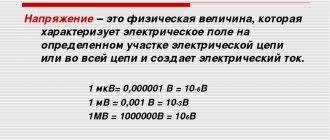
RMS value of alternating current
The value of a periodic current equal to the value of direct current, which during one period will produce the same thermal or electrodynamic effect as the periodic current, is called the effective value
periodic current:
| , | (3) |
The effective values of EMF and voltage are determined similarly.
Sinusoidally varying current
Of all the possible forms of periodic currents, the sinusoidal current is most widespread. Compared to other types of current, sinusoidal current has the advantage that it allows, in general, the most economical production, transmission, distribution and use of electrical energy. Only when using sinusoidal current is it possible to keep the shapes of voltage and current curves unchanged in all sections of a complex linear circuit. The theory of sinusoidal current is the key to understanding the theory of other circuits.
Representation of sinusoidal EMF, voltages
and currents on the Cartesian coordinate plane
Sinusoidal currents and voltages can be depicted graphically, written using equations with trigonometric functions, represented as vectors on the Cartesian plane or complex numbers.
Shown in Fig. 1, 2 graphs of two sinusoidal EMF e1
and
e2
correspond to the equations:
.
The values of the arguments of sinusoidal functions are called phases
sinusoids, and the phase value at the initial moment of time
( t =0):
and -
the initial phase
( ).
The quantity characterizing the rate of change of the phase angle is called the angular frequency.
Since the phase angle of a sinusoid
changes by rad
T f is
the frequency.
When considering two sinusoidal quantities of the same frequency together, the difference in their phase angles, equal to the difference in the initial phases, is called the phase shift angle
.
For sinusoidal EMF e1
and
e2
phase angle:
.
Vector image of sinusoidally
varying quantities
On a Cartesian plane, from the origin of coordinates, draw vectors equal in magnitude to the amplitude values of sinusoidal quantities, and rotate these vectors counterclockwise ( in TOE this direction is taken as positive
) with angular frequency equal to
w
.
The phase angle during rotation is measured from the positive semi-axis of abscissa. The projections of the rotating vectors onto the ordinate axis are equal to the instantaneous values of the emf e1
and
e2
(Fig. 3).
A set of vectors depicting sinusoidally varying emfs, voltages and currents is called vector diagrams.
When constructing vector diagrams, it is convenient to locate the vectors for the initial moment of time
( t = 0),
which follows from the equality of the angular frequencies of sinusoidal quantities and is equivalent to the fact that the Cartesian coordinate system itself rotates counterclockwise at a speed
w
. Thus, in this coordinate system the vectors are stationary (Fig. 4). Vector diagrams have found wide application in the analysis of sinusoidal current circuits. Their use makes circuit calculations more clear and simple. This simplification lies in the fact that addition and subtraction of instantaneous values of quantities can be replaced by addition and subtraction of the corresponding vectors.
Let, for example, at the branch point of the circuit (Fig. 5) the total current is equal to the sum of the currents and two branches:
.
Each of these currents is sinusoidal and can be represented by the equation
And .
The resulting current will also be sinusoidal:
.
Determining the amplitude and initial phase of this current by means of appropriate trigonometric transformations turns out to be quite cumbersome and not very visual, especially if a large number of sinusoidal quantities are summed. This is much easier to do using a vector diagram. In Fig. Figure 6 shows the initial positions of the current vectors, the projections of which onto the ordinate axis give the instantaneous current values for t=0.
When these vectors rotate with the same angular velocity
w,
their relative position does not change, and the phase shift angle between them remains equal.
Since the algebraic sum of the projections of vectors onto the ordinate axis is equal to the instantaneous value of the total current, the vector of the total current is equal to the geometric sum of the current vectors:
.
Plotting a vector diagram to scale allows you to determine the values of and from the diagram, after which a solution for the instantaneous value can be written by formally taking into account the angular frequency: .
Representation of sinusoidal EMF, voltages and currents by complex numbers
Geometric operations with vectors can be replaced by algebraic operations with complex numbers, which significantly increases the accuracy of the results obtained.
Each vector on the complex plane corresponds to a certain complex number, which can be written in:
indicative
trigonometric
or
algebraic
-
forms.
For example, EMF shown in Fig. 7 by a rotating vector, corresponds to a complex number
.
The phase angle is determined by the projections of the vector on the axes “+1” and “+j” of the coordinate system, as
.
In accordance with the trigonometric form of notation, the imaginary component of a complex number determines the instantaneous value of a sinusoidally varying EMF:
| , | (4) |
It is convenient to represent a complex number as the product of two complex numbers:
| , | (5) |
Parameter corresponding to the vector position for t =0
(or on a complex plane rotating at speed
w
), is called
the complex amplitude:
, and the parameter is
the complex of the instantaneous value.
The parameter is the rotation operator
vector by angle
wt
relative to the initial position of the vector.
Generally speaking, multiplying a vector by the rotation operator is its rotation relative to its original position by an angle ± a
.
Therefore, the instantaneous value of the sinusoidal quantity is equal to the imaginary part without the sign “ j”
product of the amplitude complex and the rotation operator:
.
The transition from one form of writing a sinusoidal quantity to another is carried out using the Euler formula:
| , | (6) |
If, for example, the complex voltage amplitude is given as a complex number in algebraic form:
,
- then to write it in exponential form, it is necessary to find the initial phase, i.e. the angle formed by the vector with the positive semi-axis +1:
.
Then the instantaneous voltage value:
,
Where .
When writing the expression, for definiteness it was assumed that , i.e. that the image vector is in the first or fourth quadrants. If , then at (second quadrant)
| , | (7) |
and at (third quadrant)
| (8) |
or
| (9) |
If the instantaneous value of the current is given in the form , then the complex amplitude is written first in exponential form, and then (if necessary) using Euler’s formula, they proceed to the algebraic form:
.
It should be noted that when adding and subtracting complexes, you should use the algebraic form of writing them, and when multiplying and dividing, the exponential form is convenient.
So, the use of complex numbers allows us to move from geometric operations on vectors to algebraic operations on complexes. So, when determining the complex amplitude of the resulting current from Fig. 5 we get:
Where ;
.
Effective value of sinusoidal EMF, voltages and currents
In accordance with expression (3), for the effective value of the sinusoidal current we write:
.
A similar result can be obtained for sinusoidal emfs and voltages. Thus, the effective values of sinusoidal current, EMF and voltage are less than their amplitude values by a factor of:
| . | (10) |
Since, as will be shown below, energy calculations of alternating current circuits are usually carried out using effective values of quantities, by analogy with the previous one we introduce the concept of an effective value complex
.
Literature
1. Basics
circuit theory: Textbook. for universities /G.V. Zeweke, P.A. Ionkin, A.V. Netushil, S.V. Strakh. –5th ed., revised. –M.: Energoatomizdat, 1989. -528 p.
2. Bessonov L.A.
Theoretical foundations of electrical engineering: Electric circuits. Textbook for students of electrical engineering, energy and instrument engineering specialties of universities. –7th ed., revised. and additional –M.: Higher. school, 1978. –528 p.
Test questions and tasks
1. What is the practical meaning of depicting sinusoidal quantities using vectors?
2. What is the practical meaning of representing sinusoidal quantities using complex numbers?
3. What are the advantages of representing sinusoidal quantities using complexes compared to their vector representation?
4. For given sinusoidal functions of emf and current, write down the corresponding complexes of amplitudes and effective values, as well as complexes of instantaneous values.
5. In Fig. 5, a. Define .
Answer: .
Effective and average values of alternating current
Everything is known about alternating current if its equation or graph is given. However, in practice it is difficult to use equations or current graphs. Alternating current is usually characterized by its effective value I. When studying rectifier devices and electrical machines, average values of e are used. d.s., current, voltage.
Effective value of alternating current
When determining the effective value of alternating current, one can proceed from any of its actions in the electrical circuit (thermal, mechanical interaction of wires with currents).
In Fig. Figure 12.18 shows graphs of two currents: constant 1 and alternating 2, and the magnitude of the direct current is equal to the amplitude of the alternating current. A direct current equal to the amplitude of an alternating current will release more heat in the same circuit element at the same time, since the alternating current is less than constant during a half-cycle, and only for one instant these currents are equal.
The effective magnitude of the alternating current I is numerically equal to the magnitude of the direct current, which in the same circuit element during the period T emits the same amount of heat as the alternating current emits under the same conditions.
The effective magnitude of the alternating current I is less than the amplitude (straight line 3 in Fig. 12.18).
Rice. 12.18. To determine the effective value of alternating current
Let us determine the amount of heat generated over a period T by a direct current equal to I and an alternating current (see Fig. 12.18) in a circuit element with resistance R: By equating we find
The effective value of the periodic current is its root mean square for the period.
It can be found from equation (12.9), but for clarity we will use a graphical solution to the problem.
The root mean square value of the alternating current over a period can be represented as the square root of the sum of a very large number of ordinates of the curve i2(t), divided by the number of ordinates n: where the numerator of the radical expression represents the sum of the squares of a number of instantaneous currents during the period, n is the number of these values , tending to ∞. In Fig. Figure 12.19 shows a number of positions of the current vector Im rotating at an angular speed ω and the corresponding instantaneous currents i. These positions are marked by points 0, 1, 2, etc. on the circle that the end of the vector Im describes.
Let us consider two positions of the vector Im (marked by points 2 and 8), separated by 90° along the circle, i.e., located in the first and second quarters of the circle, respectively. Right triangles 6′-2-2′ and 6′-8-8′ are equal because their sides are equal: 2-2′ = 6′-8′ and 2′-6′ = 8-8′. From these triangles it follows:
Rice. 12.19. To determine the effective and average value of the sinusoidal current
Each position of the vector Im in the first quarter corresponds to its other position in the second, for which a similar expression can be written. Such reasoning can be carried out for another semicircle, i.e., extend it to the second half-cycle of the current, and the squares of the negative instantaneous currents will be positive, therefore, substituting this expression in (12.10), we obtain Thus, the effective value of the sinusoidal current is less than its amplitude by a factor.
The concept of effective magnitude can be extended to all sinusoidal functions and, therefore, we can talk about the effective magnitude of voltage, e. d.s.
Effective values of current and voltage are measured by electrical measuring instruments. Rated currents and voltages of electrical devices are expressed in effective quantities. Having introduced the concept of effective magnitude, in the future we will construct vector diagrams for effective quantities of voltages and currents.
The ratio of the amplitude to the effective value is called the amplitude coefficient Ka. For a sinusoidal function this coefficient is equal to ; if the current or voltage curve has a sharper shape than a sinusoid, then Ka > , otherwise Ka (with a rectangular shape Ka = 1).
Special cases of current amplitude values
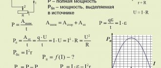
In the event that the circuit consists only of active resistance $(R)$, then:
the current coincides with the voltage in phase, the amplitude of the current in this case is equal to:
Are you an expert in this subject area? We invite you to become the author of the Directory Working Conditions
If we compare equation (6) with expression (3), we can conclude that if, instead of a capacitor, a section of the circuit is simply short-circuited, this will mean a transition to a capacitance equal to infinity.
Let the resistance $(R=0)$ be neglected in the circuit, and the capacitance be considered equal to infinity, then:
The quantity $X_L$ is called inductive reactance (inductive reactance) if it is equal to:
From the formula it follows that the inductance does not resist direct current (at $\omega$=0, $X_L$=0).
Let us assume that $R=0,\ L=0.$ Then, according to formula (3), we obtain:
The quantity $X_C=\frac{1}{\omega C}$ is called reactance capacitance (capacitance) . If the current is constant, then $X_C=\infty $. This means that no direct current flows through the capacitor.
In the event that R=0, the amplitude of the current is equal to:
Reactance (reactance) $(X)$ is a value equal to: