Electromagnetic oscillations in physics: basic formulas

The author of the article is a professional tutor, author of textbooks for preparing for the Unified State Exam Igor Vyacheslavovich Yakovlev

Topics of the Unified State Examination codifier: free electromagnetic oscillations, oscillatory circuit, forced electromagnetic oscillations, resonance, harmonic electromagnetic oscillations.

Electromagnetic vibrations

- These are periodic changes in charge, current and voltage that occur in an electrical circuit. The simplest system for observing electromagnetic oscillations is an oscillatory circuit.

Oscillatory circuit

Oscillatory circuit

is a closed circuit formed by a capacitor and a coil connected in series.

Let's charge the capacitor, connect the coil to it and close the circuit. Free electromagnetic oscillations will begin to occur

- periodic changes in the charge on the capacitor and the current in the coil. Let us remember that these oscillations are called free because they occur without any external influence - only due to the energy stored in the circuit.

The period of oscillations in the circuit will be denoted, as always, by . We will assume the coil resistance to be zero.

Let us consider in detail all the important stages of the oscillation process. For greater clarity, we will draw an analogy with the oscillations of a horizontal spring pendulum.

Starting moment

: . The capacitor charge is equal to , there is no current through the coil (Fig. 1). The capacitor will now begin to discharge.

Rice. 1.

Even though the coil resistance is zero, the current will not increase instantly. As soon as the current begins to increase, a self-induction emf will arise in the coil, preventing the current from increasing.

Analogy

. The pendulum is pulled to the right by an amount and released at the initial moment. The initial speed of the pendulum is zero.

First quarter of the period

: . The capacitor is discharging, its charge is currently equal to . The current through the coil increases (Fig. 2).

Rice. 2.

The current increases gradually: the vortex electric field of the coil prevents the current from increasing and is directed against the current.

Analogy

. The pendulum moves to the left towards the equilibrium position; the speed of the pendulum gradually increases. The deformation of the spring (aka the coordinate of the pendulum) decreases.

End of first quarter

: . The capacitor is completely discharged. The current strength reached its maximum value (Fig. 3). The capacitor will now begin recharging.

Rice. 3.

The voltage across the coil is zero, but the current will not disappear instantly. As soon as the current begins to decrease, a self-induction emf will arise in the coil, preventing the current from decreasing.

Analogy

. The pendulum passes through its equilibrium position. Its speed reaches its maximum value. The spring deformation is zero.

Second quarter

: . The capacitor is recharged - a charge of the opposite sign appears on its plates compared to what it was at the beginning (Fig. 4).

Rice. 4.

The current strength decreases gradually: the eddy electric field of the coil, supporting the decreasing current, is co-directed with the current.

Analogy

. The pendulum continues to move to the left - from the equilibrium position to the right extreme point. Its speed gradually decreases, the deformation of the spring increases.

End of second quarter

. The capacitor is completely recharged, its charge is again equal (but the polarity is different). The current strength is zero (Fig. 5). Now the reverse recharging of the capacitor will begin.

Rice. 5.

Analogy

. The pendulum has reached the far right point. The speed of the pendulum is zero. The spring deformation is maximum and equal to .

Third quarter

: . The second half of the oscillation period began; processes went in the opposite direction. The capacitor is discharged (Fig. 6).

Rice. 6.

Analogy

. The pendulum moves back: from the right extreme point to the equilibrium position.

End of the third quarter

: . The capacitor is completely discharged. The current is maximum and again equal to , but this time it has a different direction (Fig. 7).

Rice. 7.

Analogy

. The pendulum again passes through the equilibrium position at maximum speed, but this time in the opposite direction.

Fourth quarter

: . The current decreases, the capacitor charges (Fig. 8).

Rice. 8.

Analogy

. The pendulum continues to move to the right - from the equilibrium position to the extreme left point.

End of the fourth quarter and the entire period

: . Reverse charging of the capacitor is completed, the current is zero (Fig. 9).

Rice. 9.

This moment is identical to moment , and this figure is identical to Figure 1. One complete oscillation has occurred. Now the next oscillation will begin, during which the processes will occur exactly as described above.

Analogy

. The pendulum returned to its original position.

The considered electromagnetic oscillations are undamped

- they will continue indefinitely. After all, we assumed that the coil resistance is zero!

In the same way, the oscillations of a spring pendulum will be undamped in the absence of friction.

In reality, the coil has some resistance. Therefore, the oscillations in a real oscillatory circuit will be damped. So, after one complete oscillation, the charge on the capacitor will be less than the original value. Over time, the oscillations will completely disappear: all the energy initially stored in the circuit will be released in the form of heat at the resistance of the coil and connecting wires.

In the same way, the oscillations of a real spring pendulum will be damped: all the energy of the pendulum will gradually turn into heat due to the inevitable presence of friction.

Oscilloscope

But if vibrations of physical bodies are easy to observe, then vibrations of the electromagnetic field cannot be detected without special instruments. After all, it is impossible to see changes in charge, current or voltage. Using electrical measuring instruments (galvanometers, voltmeters or ammeters) for this is also inconvenient, since electromagnetic oscillations occur with a much higher frequency compared to mechanical ones. Therefore, a device called an oscilloscope .

The oscilloscope, the diagram of which you see below, is a cathode ray tube. A narrow beam of electrons passes through it and hits the screen, which begins to glow when bombarded with electrons.

An alternating sawtooth sweep voltage up is applied to the horizontally deflected plates of the tube (see figure below). It rises slowly and falls quickly. Therefore, the electric field between the plates causes the electron beam to travel horizontally across the screen at a constant speed and then return almost instantly. After this, the whole process is repeated.

If you attach the vertically deflecting plates of the tube to the capacitor, then voltage fluctuations during its discharge will cause the beam to oscillate in the vertical direction. As a result, a time sweep of oscillations is formed on the oscilloscope screen. It resembles a sine or cosine wave, similar to the one with which mechanical vibrations can be described.

Over time, electromagnetic oscillations fade. Such vibrations are free . Let us recall that free oscillations are those oscillations that occur in an oscillatory system after it is removed from an equilibrium position. In our case, the system is thrown out of equilibrium when a charge is imparted to the capacitor. Charging a capacitor is equivalent to the deviation of a mathematical pendulum from its equilibrium position.

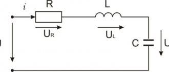
forced oscillations in an electrical circuit , which will occur as long as a periodic external force acts on the oscillatory system. Forced electromagnetic oscillations are called oscillations in a circuit under the influence of an external periodic electromotive force.

Energy transformations in an oscillatory circuit

We continue to consider undamped oscillations in the circuit, considering the coil resistance to be zero. The capacitor has a capacitance and the inductance of the coil is equal to .

Since there are no heat losses, energy does not leave the circuit: it is constantly redistributed between the capacitor and the coil.

Let's take a moment in time when the charge of the capacitor is maximum and equal to , and there is no current. The energy of the magnetic field of the coil at this moment is zero. All the energy of the circuit is concentrated in the capacitor:

Now, on the contrary, let’s consider the moment when the current is maximum and equal to , and the capacitor is discharged. The energy of the capacitor is zero. All the circuit energy is stored in the coil:

At an arbitrary moment in time, when the charge of the capacitor is equal and current flows through the coil, the energy of the circuit is equal to:

Thus,

(1)

Relationship (1) is used to solve many problems.

Electromechanical analogies

In the previous leaflet about self-induction, we noted the analogy between inductance and mass. Now we can establish several more correspondences between electrodynamic and mechanical quantities.

For a spring pendulum we have a relationship similar to (1):

(2)

Here, as you already understood, is the spring stiffness, is the mass of the pendulum, and is the current values of the coordinates and speed of the pendulum, and is their greatest values.

Comparing equalities (1) and (2) with each other, we see the following correspondences:

(3)

(4)

(5)

(6)

Based on these electromechanical analogies, we can foresee a formula for the period of electromagnetic oscillations in an oscillatory circuit.

In fact, the period of oscillation of a spring pendulum, as we know, is equal to:

In accordance with analogies (5) and (6), here we replace mass with inductance, and stiffness with inverse capacitance. We get:

(7)

Electromechanical analogies do not fail: formula (7) gives the correct expression for the period of oscillations in the oscillatory circuit. It's called Thomson's formula

. We will present its more rigorous conclusion shortly.

Harmonic law of oscillations in a circuit

Recall that the oscillations are called harmonic

, if the oscillating quantity changes over time according to the law of sine or cosine. If you have forgotten these things, be sure to repeat the “Mechanical Vibrations” sheet.

The oscillations of the charge on the capacitor and the current in the circuit turn out to be harmonic. We will prove this now. But first we need to establish rules for choosing the sign for the capacitor charge and for the current strength - after all, when oscillating, these quantities will take on both positive and negative values.

First we choose the positive traversal direction

contour.
The choice does not matter; let this direction be counterclockwise
(Fig. 10).

Rice. 10. Positive bypass direction

Current strength is considered positive if the current flows in a positive direction. Otherwise, the current will be negative.

The charge of a capacitor is the charge of the plate on which

positive current flows (i.e., the plate to which the bypass direction arrow points).
In this case, the charge on the left
plate of the capacitor.

With such a choice of signs of current and charge, the following relation is valid: (with a different choice of signs it could happen). Indeed, the signs of both parts coincide: if , then the charge of the left plate increases, and therefore .

The quantities and change over time, but the energy of the circuit remains unchanged:

(8)

Therefore, the derivative of energy with respect to time becomes zero: . We take the time derivative of both sides of relation (8); do not forget that complex functions are differentiated on the left (If is a function of , then according to the rule for differentiating a complex function, the derivative of the square of our function will be equal to: ):

Substituting and here, we get:

But the current strength is not a function that is identically equal to zero; That's why

Let's rewrite this as:

(9)

We have obtained a differential equation of harmonic oscillations of the form , where . This proves that the charge on the capacitor oscillates according to a harmonic law (i.e., according to the law of sine or cosine). The cyclic frequency of these oscillations is equal to:

(10)

This quantity is also called natural frequency

contour;
It is with this frequency that free (or, as they also say, natural
oscillations) occur in the circuit. The oscillation period is equal to:

We again come to Thomson's formula.

The harmonic dependence of charge on time in the general case has the form:

(11)

The cyclic frequency is found using formula (10); the amplitude and initial phase are determined from the initial conditions.

We will look at the situation discussed in detail at the beginning of this leaflet. Let the charge of the capacitor be maximum and equal (as in Fig. 1); there is no current in the circuit. Then the initial phase is , so that the charge varies according to the cosine law with amplitude:

(12)

Let's find the law of change in current strength. To do this, we differentiate relation (12) with respect to time, again not forgetting about the rule for finding the derivative of a complex function:

We see that the current strength also changes according to the harmonic law, this time according to the sine law:

(13)

The amplitude of the current is:

The presence of a “minus” in the law of current change (13) is not difficult to understand. Let's take, for example, the time interval (Fig. 2).

The current flows in the negative direction: . Since , the oscillation phase is in the first quarter: . The sine in the first quarter is positive; therefore, the sine in (13) will be positive on the time interval under consideration. Therefore, to ensure that the current is negative, the minus sign in formula (13) is really necessary.

Now look at fig. 8. Current flows in the positive direction. How does our “minus” work in this case? Figure out what's going on here!

Let us depict graphs of charge and current fluctuations, i.e. graphs of functions (12) and (13). For clarity, let us present these graphs in the same coordinate axes (Fig. 11).

Rice. 11. Graphs of charge and current fluctuations

Please note: charge zeros occur at current maxima or minima; conversely, current zeros correspond to charge maxima or minima.

Using the reduction formula

Let us write the law of current change (13) in the form:

Comparing this expression with the law of charge change, we see that the current phase, equal to, is greater than the charge phase by an amount. In this case, they say that the current is ahead of phase

charge on ;
or the phase shift
between current and charge is equal to ;
or the phase difference
between current and charge is equal to .

The advance of the charge current in phase is graphically manifested in the fact that the current graph is shifted to the left

on relative to the charge graph. The current strength reaches, for example, its maximum a quarter of a period earlier than the charge reaches its maximum (and a quarter of a period exactly corresponds to the phase difference).

Coil self-resonance frequency

At the dawn of the development of radio engineering, it was discovered that the coil was not an ideal inductor. At a certain frequency it enters the resonance mode even in the absence of external capacitance, and above this frequency the impedance of the coil is already capacitive in nature. To explain this phenomenon, it was assumed that in addition to inductance, a real coil also has its own capacitance (presumably between adjacent turns) and the real coil began to be represented as a model of lumped RLC elements, in which L is the inductance, C is its own capacitance, called parasitic, and with using active R, various losses in the coil are taken into account. This coil model has one resonant frequency, which is called the natural resonance frequency. For a long time this model suited everyone and became the classic model of a real coil in all textbooks.

After all, coils in the vast majority of practical applications operate at frequencies much lower than their own resonance frequency, and the designer’s task is, in fact, to ensure this condition. At the same time, most engineers for this purpose tried to reduce this very “interturn” parasitic capacitance. If the coil operates at frequencies close to its own resonance, as for example in spiral resonators or Tesla coils, the RLC model gives incorrect results, but for such cases alternative calculation algorithms were developed and everyone was satisfied without really thinking about the reasons for such inconsistencies . In our digital era, programs have appeared that make it possible to simulate the behavior of any high-frequency devices with a high degree of accuracy - so-called electromagnetic simulators. These are powerful packages like CST Studio , HFSS and many others. Let's do a study on a single layer helical coil using HFSS. In the first model, we will place the coil over an ideal conducting surface and power it from a point source with an internal resistance of 50 MΩ. The other end of the coil is grounded. The calculation will be carried out in HFSS Design mode, using the finite element method.

The second coil will be calculated using the HFSS Design-IE method, which uses the method of moments. Unlike simulators based on the NEC core, popular among radio amateurs, for example MMANA, here the segmentation is not into sections of wire, but along its surface into elementary triangular areas. With such segmentation, successful calculation requires at least 8-16 GB of computer RAM. We power the coil through short leads from the same source. Since the coil is not grounded, in this model the first resonance is half-wave.

As a result of the study, we obtained graphs of impedance at the source terminals versus frequency. The graphs show that the coil has not one, but many resonances. From this it follows that our coil is not at all a single LC circuit with its own inductance and parasitic capacitance in the form of lumped elements, as is commonly believed, but a long line with distributed parameters. This line consists of one wire, but this should not confuse anyone. The fact that wave resonance phenomena are observed even in a single wire is well illustrated by the example of a half-wave Hertz vibrator. After all, wave phenomena both in long lines and in a vibrator reflect the fact that electromagnetic interaction propagates at a finite speed. It takes a certain time for the electromagnetic interaction to “reach” from one end of the wire to the other, and when this time is comparable to the period of oscillation of the operating frequency, resonance phenomena occur. And the coil in this regard is not far from the vibrator, since despite its small dimensions, the length of the wire with which it is wound can be comparable to the wavelength. We can quite easily determine the frequency of the vibrator’s own resonance by knowing its length, taking into account the shortening coefficient. In the coil, in addition, it is necessary to take into account the connection between the turns.

In textbooks on electrodynamics [1] you can find a description of the operation of spiral waveguides with surface electromagnetic (EM) waves propagating along the spiral wire. Such waveguides are used as slow-wave structures in helical antennas and traveling wave lamps. The length of one turn and the winding pitch are comparable to the wavelength. In particular, for a spiral antenna, the turn length L is equal to the wavelength, and the winding pitch p is equal to a quarter of the wavelength. The phase velocity of the wave along the axis of the spiral waveguide is significantly lower than the speed of light, which is what its use as a slow-wave structure is based on.

[1]

Where:

vax is the wave speed along the spiral axis
c - speed of light

The relative phase velocity of the wave along the axis of such a waveguide depends only on the geometry of the spiral and does not depend on frequency, since the influence of the turns on each other is minimal and the EM wave propagates along the wire of such a spiral, just like in a vibrator. Note that the phase velocity of the EM wave relative to the spiral wire in such a waveguide is close to the speed of light.

In our coil, the length of an individual turn, and even the length of the entire winding, and even more so, the winding pitch is much less than the wavelength. In this case, in addition to the fundamental mode in such a spiral waveguide, there are higher vibration modes propagating directly along its axis. In other words, the EM wave not only propagates along the length of the wire, but part of it “jumps from turn to turn.” The relative phase velocity along the coil axis is determined by the following approximate expression:

[2]

Where:

λ0 is the wavelength of the operating frequency in free space

As can be seen from the formula, the speed depends on the diameter of the coil, the winding pitch and the wavelength. Essentially, the coil is the same spiral waveguide with slow waves, but operating in a different oscillation mode. To avoid various speculations, we note the fact that due to the presence of higher modes, the wave “gets” to the other end of the coil faster than directly along the wire. Therefore, the phase speed of the wave relative to the wire is higher than the speed of light, and by several times. This does not contradict the theory of relativity. It is enough to mention that in hollow waveguides the phase velocity of the wave is also higher than the speed of light. To understand this apparent paradox, one must distinguish between the phase and group velocities of an electromagnetic wave. Why am I referring you to textbooks...

A coil with one end grounded resonates at frequencies nλ0/4 , where n is an integer, λ0 is the wavelength of the operating frequency and fsrf = vax/λ0 . Therefore, an increase in the natural resonance frequency comes down to an increase in the value of vax . Due to the presence of higher modes of the EM wave, the frequency of the first resonance of the coil is always higher than the frequency calculated based on the length of the wire. For the same reason, the highest frequency resonances are not multiples of the first and each other. When changing the winding pitch, vax has a maximum at a spiral pitch approximately equal to the winding radius (radius a = D / 2). However, coils with a large winding pitch (p ≈ a) are not of practical interest, since they have low inductance. As the winding pitch increases, the self-resonance frequency of the coil increases (at p < a), but this increase occurs due to a decrease in the inductance value. With a fixed inductance, if we increase the winding pitch, we have to add turns and we get practically no gain.

For short coils on large-diameter frames, subsequent resonances are far higher in frequency from the first, as can be seen from the results of HFSS simulation:

At frequencies much lower than the frequency of the first resonance, the spatial delays are much less than the oscillation period, the EM field around the coil is the field of the solenoid, and the speed of wave propagation along its axis can be ignored. In this case, the RLC model of lumped elements will be quite working and fairly accurately reflect the behavior of the coil. You just have to remember that the parasitic self-capacitance is not at all the static capacitance between the turns. Coils from all three of our models in the HF range and below operate in this mode. However, already at the frequency of the first resonance, wave effects associated with the limited transmission speed of electromagnetic interactions begin to appear and the coil should be considered only as a spiral waveguide. In this case, the RLC model is not only unsuitable for calculations, but also leads to an incorrect understanding of the very mechanism of the occurrence of resonance phenomena in the coil. In this regard, I would like to note the presence on the Internet of a false idea that both wave resonance and LC resonance simultaneously occur in the coil on concentrated inductance and the notorious “interturn capacitance”. This statement is equivalent to the fact that there are two mechanisms for the propagation of electromagnetic interactions in the coil. One occurs, as usual, at the speed of light and determines the wave resonance. The second is carried out instantly with infinite speed in the virtual lumped elements of the coil. After all, the phase shift between current and voltage in reactive elements is not at all the spatial delay we are talking about. In fact, a coil, as a set of lumped RLC elements, and a coil, as a circuit with distributed parameters, are two different mathematical models of the same real coil. The first model does not take into account the limited speed of transmission of interactions; it is based on the assumption that the current density in all turns is always the same, which does not occur with the spiral’s own resonance. Therefore, this model is limited and only applicable at low frequencies. The second model is more complete, takes into account what the first did not take into account and is applicable at any frequency. There is nothing unusual about this. Any circuit whose physical dimensions are comparable to the wavelength cannot be considered as a lumped element circuit, which does not take into account the limited transmission speed of electromagnetic interactions. It is for this reason, and at the same time, by the way, the abstract mathematical concept of “inductance” itself. Like positive reactivity.

I would especially like to note the following point. At low frequencies, where, as we found out, the RLC model is valid, we can assume that both the inductance and the self-capacitance of the coil do not depend on frequency, but are determined only by the winding geometry. This is a well-known fact, which is recorded, for example, in the Nagaoka formula. However, in reality the parameters of a long spiral line depend on frequency. Not only vax , but also linear capacitance and linear inductance and, as a consequence, the values of the self-inductance and self-capacitance of the coil as a whole. Only at low frequencies is this dependence negligible, but already at frequencies close to the first resonance, the values of the inductance and self-capacitance of the coil begin to noticeably “float” in frequency. As a result, we are faced with the situation that these values, measured or calculated at low frequencies, are not suitable for calculating the self-resonance frequency of the coil as LC resonance using Thomson's formula. The calculation will give an incorrect result! Unfaithful, Karl! Thus, we come to the conclusion that calculations based on the concept of LC resonance in a coil completely lose their meaning, which once again proves the inconsistency of the RLC model of a coil not only for explaining physical phenomena at its own resonance, but also for calculations in this frequency domain. Therefore, we have to resort to a more complex numerical method from [5], which includes Bessel functions and other harsh ones, which is what Coil32 .

As can be seen from the HFSS models, both the first resonance of the coil and all subsequent resonances are associated exclusively with wave phenomena in the coil. Practical cases are possible when the coil operates in the frequency range, which includes not only its first resonance, but also higher ones. This case is described very well in I. Goncharenko’s article on the anode choke of a short-wave transmitter [2]. This example clearly shows that to correctly understand the mechanism of resonance phenomena in a coil, it is necessary to use the theory of long lines.

In addition to the phase velocity of the wave in the coil, the self-resonance frequency is influenced by the so-called end effect, similar to the well-known analogous concept from antenna theory, on which the shortening coefficient of the vibrator depends. This effect occurs because the EM field around the coil occupies a larger space than the coil itself. The presence of the end effect reduces the resonant frequency and this effect is more pronounced in short coils with a large diameter, which once again confirms the related relationship between the resonant phenomena in the coil and in the vibrator. Taking into account the phase velocity along the axis of the coil and the phenomenon of the end effect, we can calculate the self-resonance frequency of the coil using the following very approximate formula from G3RBJ:

[3]

Where:

fsrf – self-resonance frequency [MHz]
ĺw – coil wire length taking into account the end effect [m]
lw – actual coil wire length [m]
D, p, l - diameter, pitch and winding length, respectively [m]
0,25 - coefficient determining quarter-wave resonance (for half-wave resonance - 0.5)

If a designer needs to create a coil that has minimal dimensions and a maximum self-resonance frequency for a given inductance, then the most optimal would be winding with a distance between turns equal to the diameter of the wire, with a ratio l/D ≈ 1..1.5. I would like to draw the attention of designers that here we are talking about calculating the natural resonant frequency of a “bare coil in a vacuum”, i.e. one wire spiral without taking into account the influence of the frame, core, screen, wire insulation, etc. All these factors, difficult to take into account, lead to a decrease in this frequency. Moreover, everything has an impact - any conductor, printed circuit board, design body. In our HFSS models, the influencing factors are the spiral terminals and especially the solid ground in the 1st and 3rd models. Even if you decide to measure the self-resonant frequency experimentally, this will be a difficult task, since the probes of the measuring equipment also have an effect, even if the coil is hanging somewhere in the air!

It should be noted that there is no strict analytical solution to Maxwell’s equations for a cylindrical wire spiral; therefore, in theory, a spiral waveguide is represented as an equivalent model of a thin-walled solid cylinder with anisotropic conductivity. However, numerical methods for solving Maxwell’s equations (which is what HFSS basically does) lead us to quite unambiguous results. As a result, it should be borne in mind that the above simple analytical formula [3] is very approximate and cannot be applied to any coil with an arbitrary winding geometry. Therefore, in Coil32, the calculation of the natural resonance frequency is based not on the analytical, but on the numerical method from [5], which is verified by practical measurements. This does not take into account the influence of the screen, frame and other factors. The calculation has an accuracy of about 10% at 0.04 < l/D < 40. For some coils, for example for very long solenoids with a large number of turns, this method may give an incorrect result. In practice, the following simple condition must be adhered to: if the length of the wire with which the coil is wound is less than a quarter of the wavelength at the highest operating frequency, then the coil will operate below its first resonance.

PS: In conclusion, I would like to add a few words about the concept of "". This concept is based on three fundamentally false premises and is therefore fundamentally incorrect:

Any linear closed electrical circuit can be represented as a set of lumped RLC elements. The basic laws of this chain are Ohm's and Kirchhoff's laws. Any change in the topology of the circuit or the addition of elements to it completely changes the distribution of currents and voltages in the entire circuit. However, in the concept of “double resonance”, a long line is considered a kind of “black box”, equivalent to some special fourth concentrated element, the wave processes within which exist on their own. But do not forget that another name for a long line is a line with distributed parameters, when it is represented as a chain of an infinite number of RLC elements. The same laws of Ohm and Kirchhoff are also valid in it, only presented already in. We simply moved to a higher level of mathematical abstraction, which takes into account the space-time delays of the signal, but this does not change the essence of the matter. Therefore, if we connect a lumped capacitance parallel to such a line and assume that the nature of the distribution of currents and voltages within the line itself will not change, we simply deny the laws of Ohm and Kirchhoff themselves. At the same time, we must not forget that the nature of the propagation of an EM wave in a line and the nature of the distribution of currents and voltages in it are strictly interconnected things. Conclusion - wave processes in a line are not some special property of it that exists on its own, regardless of the general laws of electrical circuits. These laws are so fundamental that to a certain extent they are reflected at an even higher level of mathematical abstraction in, which describe the properties of the electromagnetic wave itself. Bottom line: “Capacitance C1 has almost no effect on the wave process” is a false statement.
“By folding a line into a spiral, little changes.” This statement is incorrect. At least the inductance increases significantly, otherwise why turn it off? In addition, the linear capacitance and linear inductance of such a line already become dependent on frequency. As a result, as noted above, Thomson’s formula for calculating the frequency of natural resonance in a spiral line ceases to work.
As a result, based on these incorrect premises, the existence of two independent resonances is asserted and two formulas are rolled out to us. Thomson's formula, which actually does not work in this case, and the formula from Alane Payne (G3RBJ), which, as we noted above, is very approximate. And according to these two formulas, the “theory of two independent resonances” is already being developed, which do not exist in reality, which is confirmed by calculations in HFSS and. I repeat once again - it’s all about different mathematical models of one real coil and different levels of mathematical abstractions depending on the specific conditions of the calculation. It is impossible to mix all this into one heap and fit it into a fictitious theory.