Electrical impulses and their parameters
An electric pulse as a deviation of voltage or current from some constant level (in particular, from zero), observed for a time less than or comparable to the duration of transient processes in the circuit.
As already mentioned, a transient process is understood as any sudden change in the steady state in an electrical circuit due to the action of external signals or switching within the circuit itself. Thus, the transient process is the process of transition of an electrical circuit from one stationary state to another. No matter how short this transition process is, it is always finite in time. For circuits in which the lifetime of the transient process is incomparably less than the time of action of the external signal (voltage or current), the operating mode is considered to be steady, and the external signal itself for such a circuit is not pulsed. An example of this is the operation of an electromagnetic relay.
When the duration of the voltage or current signals operating in an electrical circuit becomes commensurate with the duration of the establishment processes, the transient process has such a strong influence on the shape and parameters of these signals that they cannot be ignored. In this case, most of the time the signal influences the electrical circuit coincides with the lifetime of the transient process (Fig. 1.4). The operating mode of the circuit during the action of such a signal will be non-stationary, and its effect on the electrical circuit will be pulsed.
\
a) b)
Fig.1.4. The relationship between signal duration and duration
transition process:
a) the duration of the transition process is significantly less than the duration
signal ( τpp << t );
b) the duration of the transition process is commensurate with the duration
signal ( τpp ≈ t ).
It follows that the concept of a pulse is associated with the parameters of a specific circuit and that not for every circuit the signal can be considered pulsed.
Thus, an electrical pulse for a given circuit is a voltage or current acting for a period of time commensurate with the duration of the transient process in this circuit. In this case, it is assumed that there must be a sufficient period of time between two pulses acting sequentially in the circuit, exceeding the duration of the establishment process. Otherwise, signals of complex shapes will appear instead of pulses (Fig. 1.5).
Fig.1.5. Electrical signals of complex shapes
The presence of time intervals gives the pulse signal a characteristic intermittent structure. Some convention of such definitions lies in the fact that the establishment process theoretically lasts indefinitely.
There may be such intermediate cases when transient processes in circuits do not have time to practically end from pulse to pulse, although the acting signals continue to be called pulsed. In such cases, additional distortions in the pulse shape occur, caused by the superposition of the transient process on the beginning of the subsequent pulse.
There are two types of pulses: video pulses and radio pulses . Video pulses are received when commutating (switching) a DC circuit. Such pulses do not contain high-frequency oscillations and have a constant component (average value) different from zero.
Video pulses are usually distinguished by their shape. In Fig. 1.6. the most frequently occurring video pulses are shown.
Rice. 1.6. Video pulse shapes:
a) rectangular; b) trapezoidal; c) pointed;
d) sawtooth; e) triangular; e) heteropolar.
Let's consider the main parameters of a single pulse (Fig. 1.7).
Rice. 1.7. Single pulse parameters
The shape of the pulses and the properties of its individual sections are quantitatively assessed by the following parameters:
· Um – amplitude (maximum value) of the pulse. The pulse amplitude Um (Im) is expressed in volts (amps).
· τ and – pulse duration. Typically, measurements of the duration of pulses or individual sections are made at a certain level from their base. If this is not specified, then the pulse duration is determined at the zero level. However, most often the pulse duration is determined at the level of 0.1 Um or 0.5 Um , counting from the base. In the latter case, the pulse duration is called active duration and is denoted τ ia . If necessary and depending on the shape of the pulses, the accepted level values for measurement are specially specified.
· τф – front duration, determined by the rise time of the pulse from the level of 0.1 Um to the level of 0.9 Um .
· τс – cutoff duration (back edge), determined by the pulse decay time from the level of 0.9 Um to the level of 0.1 Um . When the rise or fall duration is measured at 0.5 Um , it is called the active duration and is designated by adding the subscript “a”, similar to the active pulse duration. Typically τph and τс are a few percent of the pulse duration. The smaller τph and τc compared to τ and , the more the pulse shape approaches rectangular. Sometimes, instead of τph and τc , the pulse fronts are characterized by the rate of rise (decay). This value is called the slope (S) of the front (cut) and is expressed in volts per second (V
/
s) or kilovolts per second (kV
/
s) .
For a rectangular pulse ……………………………(1.14).
· The section of the pulse between the fronts is called the flat top. Figure 1.7 shows the flat top decay ( ΔU) .
· Pulse power. The energy W of the pulse, related to its duration, determines the power in the pulse:
………………………………(1.15).
It is expressed in watts (W) , kilowatts (kW) or fractional units.
tsah watta.
Pulse devices use pulses with durations ranging from fractions of a second to nanoseconds (10 - 9 s) .
The characteristic sections of the pulse (Fig. 1.8), which determine its shape,
are:
· front (1 – 2);
· top (2 – 3);
· cut (3 – 4), sometimes called trailing edge;
· tail (4 – 5).
Fig.1.8. Characteristic sections of the pulse
Certain sections of pulses of different shapes may be missing. It should be borne in mind that real pulses do not have a shape that strictly corresponds to the name. There are pulses of positive and negative polarity, as well as bilateral (multipolar) pulses
(Fig. 1.6, f
).
Radio pulses are pulses of high-frequency oscillations of voltage or current, usually of a sinusoidal shape. Radio pulses do not have a constant component. Radio pulses are obtained by modulating high-frequency sinusoidal oscillations in amplitude. In this case, amplitude modulation is carried out according to the law of the control video pulse. The shapes of the corresponding radio pulses obtained using amplitude modulation are shown in Fig. 1.9:
Fig.1.9. Radio pulse shapes
Electrical pulses following each other at equal intervals of time are called a periodic sequence (Fig. 1.10).
Fig.1.10. Periodic pulse sequence
A periodic sequence of pulses is characterized by the following parameters:
· Repetition period Ti – the time interval between the beginning of two adjacent unipolar pulses. It is expressed in seconds (s) or subseconds (ms; μs; ns). The reciprocal of the repetition period is called the pulse repetition rate. It determines the number of pulses within one second and is expressed in hertz (Hz) , kilohertz (kHz) , etc.
……………………………….. (1.16)
· The duty cycle of a pulse sequence is the ratio of the repetition period to the pulse duration. Denoted by the letter q :
………………… (1.17)
The duty cycle is a dimensionless quantity that can vary over a very wide range, since the duration of the pulses can be hundreds and even thousands of times less than the pulse period or, conversely, occupy most of the period.
The reciprocal of the duty cycle is called the duty cycle. This quantity is dimensionless, less than unity. It is denoted by the letter γ :
…………………………(1.18)
A sequence of pulses with q = 2 is called a “meander” . This one has
sequences (Fig. 1.6, f
).
If Ti>> τi , then such a sequence is called radar.
· Average value (constant component) of impulse oscillation. When determining the period-average value of a pulse oscillation Uav (or Iav), the voltage or current pulse is distributed evenly over the entire period so that the area Uav ·Ti is equal to the area of the pulse Si = Um · τi (Fig. 1.10).
For pulses of any shape, the average value is determined from the expression
……………………(1.19),
where U(t) is an analytical expression for the pulse shape.
For a periodic sequence of rectangular pulses, for which U(t) = Um , repetition period Ti and pulse duration τi , this expression after substitution and transformation takes the form:
…………………….(1.20).
From Fig. 1.10 it is clear that Si = Um τi = Uav·Ti , which implies:
……………(1.21),
where U0 is called the constant component.
Thus, the average value (constant component) of the voltage (current) of a sequence of rectangular pulses is q times less than the pulse amplitude.
· Average power of the pulse sequence. The pulse energy W , related to the period Ti , determines the average pulse power
…………………………….. (1.22).
Comparing the expressions Ri and Рср , we get
Ri · τi = Рср · Ti ,
whence follows
…………………(1.23)
And
……………………. (1.24),
those. the average power and the power per pulse differ by q times.
It follows that the pulse power provided by the generator can be q times greater than the average power of the generator.
Tasks and exercises
1. Pulse amplitude is 11 kV, pulse duration is 1 μs. Determine the steepness of the pulse front, if we consider the front duration to be equal to 20% of the pulse duration.
2. The amplitude of rectangular pulses with a repetition frequency of 1250 Hz and a duty cycle of 2300 is 11 kV. Determine the slope of the front and cutoff, if we consider the duration of the front and cutoff to be equal to 20% of the pulse duration.
3. Determine the time constant of a circuit consisting of a capacitor with a capacity of 5000 pF and an active resistance of 0.5 MΩ.
4. Determine the time constant of a circuit consisting of an inductance of 20 mH and an active resistance of 5 kOhm.
5. Determine the average power of the radar transmitting device, which has the following parameters: pulse power 800 kW; probe pulse duration 3.2 μs; repetition rate of probing pulses is 375 Hz.
6. A capacitor with a capacity of 400 pF is charged from a constant voltage source of 200 V through a resistance of 0.5 MΩ. Determine the voltage across the capacitor 600 μs after the start of charging.
7. A DC source with a voltage of 50 V is connected to a circuit consisting of a capacitor with a capacity of 10 pF and a resistance of 2 MΩ. Determine the current at the moment of switching on and 40 μs after switching on.
8. A capacitor charged to a voltage of 300 V is discharged through a resistance of 300 MΩ. Determine the magnitude of the discharge current at time t = 3τ after the start of the discharge.
9. How long will it take to charge a capacitor with a capacity of 100 pF to a voltage of 340 V if the source voltage is 540 V and the resistance of the charging circuit is 100 kOhm?
10. A circuit consisting of an inductance of 10 mH and a resistance of 5 kOhm is connected to a DC voltage source of 250 V. Determine the current flowing in the circuit 4 μs after switching on.
Chapter 2. Pulse Shaping
Linear and nonlinear circuits
In pulse technology, circuits and devices are widely used that generate voltages of one form from voltages of another. Such problems are solved using linear and nonlinear elements.
An element whose parameters (resistance, inductance, capacitance) do not depend on the magnitude and direction of currents and applied voltages is called linear. Circuits containing linear elements are called
linear.
Properties of linear circuits:
· The current-voltage characteristic (volt-ampere characteristic) of a linear circuit is a straight line, i.e. the magnitudes of currents and voltages will be related to each other by linear equations with constant coefficients. An example of a current-voltage characteristic of this type is Ohm’s law: .
· For the calculation (analysis) and synthesis of linear circuits, we apply the principle of superposition (overlay). The meaning of the superposition principle is as follows: if a sinusoidal voltage is applied to the input of a linear circuit, then the voltage on any of its elements will have the same shape. If the input voltage is a complex signal (i.e., it is the sum of harmonics), then at any element of the linear circuit all the harmonic components of this signal are preserved: in other words, the shape of the voltage applied to the input is preserved. In this case, only the ratio of harmonic amplitudes will change at the output of the linear circuit.
· A linear circuit does not transform the spectrum of the electrical signal. It can change the components of the spectrum only in amplitude and phase. This is the cause of linear distortion .
· Any real linear circuit distorts the signal shape due to transients and finite bandwidth.
Strictly speaking, all elements of electrical circuits are nonlinear. However, in a certain range of changes in variable quantities, the nonlinearity of the elements manifests itself so little that it can practically be neglected. An example is a radio frequency amplifier (RFA) of a radio receiver, the input of which is supplied with a very low amplitude signal from the antenna.
The nonlinearity of the input characteristic of the transistor in the first stage of the RF amplifier, within a few microvolts, is so small that it is simply not taken into account.
Typically, the area of nonlinear behavior of an element is limited, and the transition to nonlinearity can occur either gradually or abruptly.
If a complex signal is applied to the input of a linear circuit, which is the sum of harmonics of different frequencies, and the linear circuit contains a frequency-dependent element ( L or C ), then the shape of the voltages on its elements will not repeat the shape of the input voltage. This is explained by the fact that the harmonics of the input voltage are transmitted differently by such a circuit. As a result of the input signal passing through the capacitances and inductances of the circuit, the relationships between the harmonic components on the circuit elements change in amplitude and phase relative to the input signal. As a result, the relationships between the amplitudes and phases of the harmonics at the input of the circuit and at its output are not the same. This property is the basis for the formation of pulses using linear circuits.
An element whose parameters depend on the magnitude and polarity of applied voltages or flowing currents is called nonlinear , and a circuit containing such elements is called nonlinear .
Nonlinear elements include electrovacuum devices (EVDs), semiconductor devices (SCDs) operating in the nonlinear section of the current-voltage characteristic, diodes (vacuum and semiconductor), as well as transformers with ferromagnets.
Properties of nonlinear circuits:
· The current flowing through a nonlinear element is not proportional to the voltage applied to it, i.e. The relationship between voltage and current (CV) is nonlinear. An example of such a current-voltage characteristic is the input and output characteristics of EVP and PPP.
· Processes occurring in nonlinear circuits are described by nonlinear equations of various types, the coefficients of which depend on the voltage (current) function itself or on its derivatives, and the current-voltage characteristic of a nonlinear circuit has the form of a curve or broken line. An example is the characteristics of diodes, triodes, thyristors, zener diodes, etc.
· For nonlinear circuits the principle of superpositions is not applicable. When an external signal acts on nonlinear circuits, currents always arise in them, containing new frequency components that were not in the input signal. This is the cause of
nonlinear distortion , causing the output signal to be nonlinear
the circuit always differs in shape from the input signal.
Differentiating chains
In order to obtain a pulse of the desired shape from a given voltage shape using a passive electrical circuit, it is necessary to know the forming properties of this circuit. Forming properties characterize the ability of a linear circuit to change the shape of the transmitted (processed) signal in a certain way and are completely determined by the type of its frequency and time characteristics .
In pulse technology, linear two- and four-terminal networks are widely used to generate signals.
A differentiating circuit is a circuit whose output voltage is proportional to the first derivative of the input voltage. Mathematically this is expressed by the following formula:
………………………. (2.1),
where Uin is the voltage at the input of the differentiating circuit;
Uout – voltage at the output of the differentiating circuit;
k – proportionality coefficient.
Differentiating circuits (DC) are used to differentiate video pulses. In this case, differentiating chains allow the following transformations:
· shortening of rectangular video pulses and the formation of pointed pulses from them, which serve to trigger and synchronize various pulse devices;
· obtaining time derivatives of complex functions. This is used in measuring technology, auto-regulation and auto-tracking systems;
· formation of rectangular pulses from sawtooth ones.
The simplest differentiating circuits are capacitive ( RC )
and inductive (
RL )
circuits (Fig. 2.1):
a) b)
Fig.2.1. Types of differentiating chains:
a) capacitive DC; b) inductive DC
An inductive differentiating circuit is used much less frequently than a capacitive circuit for purely practical reasons. The fact is that to fulfill the differentiation condition, a coil with high inductance is required. Such coils without iron turn out to be very bulky and have a large parasitic (interturn) capacitance, which distorts the result of differentiation. It is not advisable to use coils with iron, because the current shape is distorted due to the nonlinearity of the iron magnetization curve, as a result of which nonlinear distortions of the output signal occur during differentiation. Therefore, we will consider a capacitive differentiating circuit.
Let us show that the RC chain becomes differentiating under certain conditions.
It is known that the current flowing through the capacitance is determined by the expression:
……………………………………. (2.2).
At the same time, from Fig. 2.1, a
it's obvious that
,
because R and C represent a voltage divider. Because the voltage
, That .
Output voltage
……………………. (2.3).
Substituting expression (2.2) into (2.3), we obtain:
……………… (2.4).
If we choose a small enough value of R so that the condition is satisfied,
then we get the approximate equality
……………………….. (2.5).
This equality is identical to (2.1).
Choosing R of a sufficiently small value means ensuring the fulfillment of the inequality
, i.e. ,
where ωв = 2πfв is the upper limit frequency of the harmonic of the output signal, which is also significant for the shape of the output pulse.
The proportionality coefficient in expression (2.1) k = RC = τ is called the time constant of the differentiating chain. The sharper the input voltage changes, the smaller the value of τ the differentiating circuit must have so that the output voltage is close in shape to the derivative of Uin . The parameter τ = RC has the dimension of time. This can be confirmed by the fact that, in accordance with the International System of Units (SI), the unit of measurement for electrical resistance is
,
and the unit of measurement of electrical capacitance
.
Hence,
The principle of operation of the differentiating chain.
The schematic diagram of the capacitive differentiating circuit is shown in Fig. 2.2, and the voltage diagrams are shown in Fig. 2.3.
Fig.2.2. Schematic diagram of a capacitive differentiating circuit
Let an ideal rectangular pulse be supplied to the input, for which
τф= τс = 0 , and the internal resistance of the signal source Ri = 0. Let the pulse be determined by the following expression:
- Initial state of the circuit (t < t1).
In the initial state Uin = 0; Uc = 0; ic = 0; Uout = 0.
- First voltage surge (t = t1).
At time t = t1, a voltage jump is supplied to the input of the DC
Uin = E. At this moment Uc = 0 , because In an infinitely small period of time, the capacity cannot be charged. But, in accordance with the law of commutation, the current through the capacitance can increase instantly. Therefore, at the moment t = t1, the current flowing through the capacitance will be equal to
Therefore, the voltage at the output of the circuit at this moment will be equal to
- Capacitor charge (t1 < t < t2).
After the jump, the capacitor begins charging with a current that decreases according to an exponential law:
Fig.2.3. Stress diagrams on the elements of the differentiating circuit
The voltage across the capacitor will increase exponentially
law:
…………………… (2.6).
The DC output voltage will drop as the voltage increases
charge on the capacitor, because R and C represent a voltage divider:
…………. (2.7).
It must be remembered that at any time the voltage divider satisfies the equality
whence it follows that
,
which confirms the validity of expression (2.7).
Theoretically, the charge of the capacitor will continue indefinitely, but practically this transient process ends after
(3…5) τzare = (3…5) RC .
- End of capacitor charging (t = t2).
After the end of the transition process, the capacitor charge current becomes zero. Therefore, the voltage at the output of the differentiating circuit
reaches almost zero value, i.e. at time t = t2
- Steady state (t2 < t < t3).
Wherein
- Second voltage surge (t = t3).
At time t = t3, the voltage at the input of the differentiating circuit abruptly drops to zero. Capacitor C becomes a voltage source because it is charged to a value of .
Since, in accordance with the switching law, the voltage on the capacitor cannot change abruptly, and the current flowing through the capacitance can change abruptly, then at the moment t = t3 the output voltage decreases abruptly to – E. In this case, the discharge current at a given time becomes maximum:
,
and the voltage at the output of the differentiating circuit
.
The output voltage has a minus sign, because the current changed its direction.
- Capacitor discharge (t3 < t < t4).
After the second jump, the voltage on the capacitor begins to decrease according to the exponential law:
;
;
- The end of the capacitor discharge and restoration of the initial state of the circuit (t ≥ t4).
After the end of the transient discharge process of the capacitor
Thus, the circuit returned to its original state. The end of the capacitor discharge occurs almost at t = (3…5)τ = (3…5) RC.
Since we assumed the internal resistance of the signal source Ri = 0, we can assume that the time constants of the charge and discharge circuits of the capacitor are τcharge = τtime = τ = RC .
In such an ideal circuit, the amplitude of the output voltage Uout.max does not depend on the value of the circuit parameters R and C , and the duration of the output pulses is determined by the value of the circuit time constant τ = RC . The smaller the values of R and C , the faster the transient processes of charging and discharging the capacitance end, the shorter the pulse at the circuit output.
Theoretically, the duration of the pulse at the output of the differentiating circuit, determined by the base, turns out to be infinitely long, since the voltage at the output decreases exponentially. Therefore, the pulse duration is determined at a certain level from the base
U0 = αUout (Fig. 2.4):
Fig.2.4. Determination of the pulse duration at level U0 after
differentiation
Let us determine the duration of the differentiated pulse at the level
U0 = αUout :
………………. (2.8),
from where and
……………………… (2.9).
Differentiation is always accompanied by a shortening of the pulse duration. This means that the capacitance C must have time to fully charge during the current input differentiable pulse. Therefore, the condition for practical differentiation in order to shorten the pulse duration is the relationship:
τi input > 5τ = 5RC.
The smaller the τ of the circuit, the faster the capacitor charges and discharges and the shorter the duration of the output pulses, the more pointed they become and, therefore, the more accurate the differentiation. However, it is advisable to reduce τ to a certain limit.
The change in the pulse shape at the output of the differentiating circuit can be explained from the point of view of spectral analysis.
Each harmonic of the input pulse is divided between R and C. For harmonics of low frequencies, which determine the top of the input pulse, the capacitor represents a large resistance, because
>> R.
Therefore, the flat top of the input pulse is almost not transmitted to the output.
For high-frequency components of the input pulse, forming its front and tail,
<< R.
Therefore, the front and tail of the input pulse are transmitted to the output practically without attenuation. These considerations allow the differentiating circuit to be defined as a high-pass filter .
Transition process
Consideration of pulsed devices and circuits is not possible without an understanding of the transient process. It occurs in circuits during various switchings, that is, when turning on or off circuit elements, voltage sources, short circuits of individual circuits, etc. The transient process is explained by the fact that the energy of the electromagnetic fields associated with the circuit is not the same at different periods of time, and a sharp change in energy is impossible due to the limited power of the power sources.
Based on the above, we can conclude that the voltage across the capacitor and the current into the inductor cannot change abruptly, since these parameters determine the energy of the electric field of the capacitor and the magnetic field of the inductor.
Thus, we can conclude that when considering pulsed circuits, the greatest attention should be paid to circuits that are combinations of resistors and capacitors or resistors and inductors (RC and RL circuits). Such circuits are used directly for generating pulses, and are also the most important elements of relaxation generators, triggers and other devices. Therefore, below we will consider the basic properties of elementary RC and RL circuits, as well as the change in the shape of pulses when passing through these circuits.
The influence of RC and RL circuits on pulses of various shapes
Despite the fact that the shapes of electrical pulses are quite diverse, they can be represented as a sum of elementary (typical) voltages of three forms: abrupt, linearly varying and exponential. Therefore, we will consider the effect of various voltage forms on RC and RL circuits.
Illustration of RC and RL circuits.
Elementary forms of voltage (from top to bottom): stepwise, linearly varying, exponential.
Voltage step change
. When connecting an RC circuit to a constant voltage source uin = E = const, the voltage on the capacitor and resistor will change according to an exponential law:
where e is a mathematical constant, e = 2.72; t – time, s; τ
– time constant, s.
τ = RC
.
Everything is clear with the definition of voltage, but in practice the question more often arises about the time of voltage establishment. For example, it is necessary to calculate the time during which a voltage equal to uC = 0.95 E is established on the capacitor. By simply transforming the voltage formula, we get
Similarly, when connecting an RL circuit to a constant voltage source uin = E = const
where τ
– time constant, s.
τ = L/R
.
Voltage ramp
. When connecting an RC circuit to a source of linearly varying voltage uВХ = kt, the voltages on the resistor and capacitor will change according to the following formula
For an RL circuit connected to a source with a linearly varying voltage uВХ = kt, the voltages on the elements will accordingly be as follows
Voltage timing diagrams for linearly varying voltage in RC and RL circuits.
Exponentially varying voltage. When connecting an RC circuit to an exponentially varying voltage source, the voltages across the resistor and capacitor will change according to the following formula
where q = τ/τ1.
Accordingly, the voltage across the capacitor will be equal to the difference between the source voltage and the voltage across the resistor
Timing diagrams for uR are presented below for various values of q. At large values of q, that is, the circuit time constant τ, the voltage shapes uR are close to the shapes corresponding to a step change in the input voltage. As τ decreases, in addition to reducing the duration of the voltage drop uR, the maximum value uR also decreases.
Time diagrams of voltages across a resistor of an RC circuit at various values of q = τ/τ1.
The formulas and timing diagrams for the voltages at the output of the RL circuit turn out to be the same as for the RC circuit.