Various physical, chemical, economic and even social phenomena are characterized by a reaction delay effect. This phenomenon occurs as a result of a reaction to a certain irritation, action or influence. The article will give a detailed description of what hysteresis is. Describes its most common variants, the influence of this effect in electrical engineering and electronics.
Magnetic hysteresis
This is an irreversible and ambiguous dependence of the magnetization index of a substance (and these are, as a rule, magnetically ordered ferromagnets) on an external magnetic field. In this case, the field is constantly changing - decreasing or increasing. The general reason for the existence of hysteresis is the presence at the minimum of the thermodynamic potential of an unstable state and a stable one, and there are also irreversible transitions between them. Hysteresis is also a manifestation of a first-order magnetic orientational phase transition. With them, transitions from one to another phases occur due to metastable states. The characteristic is a graph called the “hysteresis loop”. Sometimes it is also called the “magnetization curve.”
Hysteresis in electronics
In electrical engineering and electronics, the property of hysteresis is used by devices that use various magnetic interactions. For example, magnetic storage media or a Schmitt trigger.
This property must be known in order to use it to suppress noise at the moment of switching certain logical signals (contact bounce, fast oscillations).
There are two types of elastic hysteresis: dynamic and static. In the first case, the graph will depict a constantly changing loop, in the second - a uniform one.
This phenomenon is most noticeable in precision voltage references used in instrument transducers.
Hysteresis loop
On the graph of M versus H you can see:
- From the zero state, at which M = 0 and H = 0, with increasing H, M also increases.
- When the field increases, the magnetization becomes almost constant and is equal to the saturation value.
- As H decreases, the opposite change occurs, but when H = 0, the magnetization M will not be zero. This change can be seen in the demagnetization curve. And when H=0, M takes on a value equal to the residual magnetization.
- As H increases in the range –Ht… +Ht, the magnetization changes along the third curve.
- All three curves describing the processes are connected and form a kind of loop. It describes the phenomenon of hysteresis - the processes of magnetization and demagnetization.
Magnetizing energy
The loop is considered asymmetrical in the case when the maxima of the H1 field, which are applied in the reverse and forward directions, are not the same. Above we described a loop that is characteristic of a slow process of magnetization reversal. With them, quasi-equilibrium relationships between the values of H and M are maintained. It is necessary to pay attention to the fact that during magnetization or demagnetization, M lags behind H. And this leads to the fact that all the energy that is acquired by the ferromagnetic material during magnetization is not given up completely when going through the demagnetization cycle. And this difference all goes into heating the ferromagnet. And the magnetic hysteresis loop turns out to be asymmetrical in this case.
HYSTERESIS
HYSTERESIS (from the Greek ὑστέρησις - lag, delay), delay in physical changes. quantities characterizing the state of a substance from changes in other physical. quantity that determines external conditions. G. occurs in those cases when the state of the body at a given moment in time is determined by external conditions not only at the same time, but also at previous points in time. As a result, for cyclic process (increase and decrease in external influence), a loop-shaped (ambiguous) diagram is obtained, which is called a hysteresis loop. G. arises in decomposition. substances and with different physical processes. Of greatest interest are magnetic, ferroelectric and elastic hysteresis.
Magnetic geometry is an ambiguous dependence of the magnetization $\boldsymbol M$ of a magnetically ordered substance (magnet, for example, ferro- or ferrimagnet) on the external magnetic field $\boldsymbol H$ when it is cyclic. change (increase and decrease). The reason for the existence of magnetic geometry is the presence, in a certain interval, of changes in $\boldsymbol H$ among the states of the magnet that correspond to the thermodynamic minimum. potential, metastable states (along with stable ones) and irreversible transitions between them. Magnetic hysteresis can also be considered as a manifestation of magnetic orientational phase transitions of the 1st order, for which direct and reverse transitions between phases depending on $\boldsymbol H$ occur, due to the indicated metastability of states, at decomp. values of $\boldsymbol H$.
Rice. 1. Magnetic hysteresis loops: 1 – maximum, 2 – partial; a – magnetization curve, b and c – magnetization reversal curves; МR – residual magnetization, Нс – coercive force, Ms – magnetized...
In Fig. Figure 1 schematically shows the typical dependence of $M$ on $H$ in a ferromagnet; from the state $M=0$ at $H=0$, with increasing $H$ the value of $M$ increases (main magnetization curve, $\it a$) and in a sufficiently strong field $H⩾H_{\text m}$ $M$ becomes practically constant and equal to the saturation magnetization $M_{\text s}$. As $H$ decreases from the value of $H_{\text m}$, the magnetization changes along the branch $\it b$ and at $H=0$ takes the value $M=M_{\text R}$ (residual magnetization). To demagnetize a substance ($M=0$), it is necessary to apply a reverse field $H= –H_{\text c}$, called coercive force. Then, at $H=–H_{\text m}$, the sample is magnetized to saturation ($M=–M_{\text s}$) in the opposite direction. As $H$ changes from $–H_{\text m}$ to $+H_{\text m}$, the magnetization changes along the $\it in$ curve. The branches $\it b$ and $\it c$, resulting from changing $H$ from $+H_{\text m}$ to $–H_{\text m}$ and back, form a closed curve called maximal (or limit) loop G. The branches $\it b$ and $\it c$ are called, respectively, the descending and ascending branches of the loop G. When $H$ changes on the segment $[–H_1, H_1]$ with $H_1$, the dependence of $M (H)$ is described by a closed curve (partial loop of G.), entirely lying inside the max. hysteresis loops.
The described magnetic loops are characteristic of fairly slow (quasi-static) magnetization reversal processes. The lag of $M$ from $H$ during magnetization and demagnetization leads to the fact that the energy acquired by the magnet during magnetization is not completely released during demagnetization. The energy lost in one cycle is determined by the area of the loop G. These energy losses are called hysteresis. With dynamic When a sample is remagnetized by an alternating magnetic field $\boldsymbol H_{\sim}$, the hysteresis loop turns out to be wider than the static one due to the fact that dynamic losses are added to the quasi-equilibrium hysteresis losses, which can be associated with eddy currents (in conductors) and relaxation phenomena.
The shape of the magnetic loop and the most important characteristics of the magnetic magnetic resonance (hysteresis losses, $H_с$, $M_{\text R}$, etc.) depend on the chemical. the composition of the substance, its structural state and temperature, on the nature and distribution of defects in the sample, and, consequently, on the technology of its preparation and subsequent physical. treatments (thermal, mechanical, thermomagnetic, etc.). The hysteretic behavior of a number of other physical systems is associated with magnetic hysteresis. properties, eg. G. magnetostriction, G. galvanomagnetic and magneto-optical. phenomena, etc.
Ferroelectric G. - an ambiguous dependence of the magnitude of the electrical vector. polarization $\boldsymbol P$ of ferroelectrics on the strength $\boldsymbol E$ of the external electric. fields at cyclic changing the latter. Ferroelectrics have a spontaneous (i.e., spontaneous, arising in the absence of an external field) polarization $\boldsymbol P_{sp}$ in a certain temperature range. The direction of polarization can be changed electrically. field, while the value of $\boldsymbol P$ for a given $\boldsymbol E$ depends on the prehistory, i.e., on what the electric power was like. field at previous times. Ferroelectric G. has the appearance of a characteristic loop (G.'s loop), main. the parameters of which are the residual polarization $\boldsymbol P_{res}$ at $\boldsymbol E=0$ and the coercive field $\boldsymbol E_к$, at which the direction (switching) of the vector $\boldsymbol P_{cn}$ changes. For perfect single crystals, the G. loop has a shape close to rectangular, and $\boldsymbol P_{ost}=\boldsymbol P_{sp}$. In real crystals, the residual polarization is less than spontaneous due to the division of the crystal into domains.
The existence of ferroelectric G. follows from phenomenological. ferroelectric theory phenomena, according to which the equilibrium values of $\boldsymbol P_{sp}$ at any temperature below the ferroelectric temperature. phase transition corresponds to two symmetrical thermodynamic minima. potentials separated by a potential barrier. At $E=±E_к$ one of the minima disappears, and the crystal finds itself in a state with a certain direction of the vector $\boldsymbol P_{sp}$. When cyclic switching spontaneous polarization, the area of the G. loop determines the hysteresis losses - the amount of electrical energy. field turning into heat. The magnitude of the coercive field is also associated with the processes of nucleation and evolution in electricity. ferroelectric field domains - areas of the crystal with a dedicated electrical field in the direction of the spontaneous polarization vector.
Rice. 2. Elastic hysteresis loop.
Elastic g. - an ambiguous dependence of mechanical stress on the deformation of an elastic body during cyclic. application and removal of load. The graph of stress $σ$ versus strain $ε$ differs from a straight line segment corresponding to Hooke’s law and represents a G. loop (Fig. 2). The area of this loop is proportional to the mechanical energy that was dissipated (converted to heat) during the cycle.
The appearance of elastic stress in metals is due to the fact that in some polycrystal grains microstresses significantly exceed the average stress. stress in the sample, which leads to the appearance of plastic. deformations and thereby to the dissipation of mechanical. energy. In some cases, electromagnetic phenomena make a contribution to elastic gravity.
Elastic fluidity, as a manifestation of the difference between a real elastic body and an ideally elastic one, is observed in all solids, even at very low temperatures. Elastic vibration is the reason for the damping of free vibrations of elastic bodies, the damping of sound in them, and a decrease in the coefficient. recovery during an inelastic impact, etc. In the general case, the deviation of elasticity from ideal is included in the concept of internal friction.
Hysteresis losses
During dynamic magnetization reversal of a ferromagnet by an alternating magnetic field, losses are observed. Moreover, they constitute only a small fraction of the total magnetic losses. If the loops have the same height (the same maximum magnetization value M), the dynamic type loop turns out to be wider than the static one. This happens due to the fact that new ones are added to all losses. These are dynamic losses, they are usually associated with eddy current and magnetic viscosity. In total, quite significant losses due to hysteresis are obtained.
Properties of ferromagnetic materials. Hysteresis
If the medium is capable of magnetization in a magnetic field, i.e. create its own magnetic field, then such a medium is called a magnet. In fact, if a non-magnetized magnet is placed in a magnetic field with induction , then it becomes magnetized and gives an additional field induction, which adds up vectorially to the initial induction, i.e. ´.
The vector sum is called the vector of magnetic induction inside the magnet.
Substances for which ´ coincides in direction with , are called paramagnets. Inside paramagnetic materials, the magnetic field increases.
Substances for which ´ and are opposite in direction are called diamagnetic. The magnetic field inside diamagnetic materials is weakened. For paramagnetic materials (aluminum, platinum, etc.) magnetic permeability µ>1. For diamagnetic materials (copper, table salt, etc.) µ<1.
Along with para- and diamagnets, there are ferromagnets (iron, nickel, cobalt, etc.), for which µ>>1, i.e. they are capable of being highly magnetized.
For para- and diamagnets, the relationship between and is linear, since µ=const. For ferromagnets, this dependence is nonlinear (Fig. 32), because µ≠const, and depends on H, i.e. µ=ƒ(Н) (Fig. 33).
Rice. 32 Fig. 33
A characteristic feature of ferromagnets is hysteresis. The phenomenon of hysteresis lies in the fact that magnetic induction B depends not only on the instantaneous value of H, but also on what the field strength was before. In this case, there is a lag in the change in induction B with a change in H. If a non-magnetized ferromagnet is placed in a magnetic field that increases from zero, then the dependence of B on H (magnetization curve) will be expressed by the curve Oa (Fig. 34). Point “a” in Fig. 34 corresponds to magnetic saturation.
Fig.34
If we then reduce H to 0, then the magnetization curve does not coincide with Oa, but follows the ab curve. As a result, when H becomes equal to zero, magnetization will not disappear and will be characterized by the value Be, which is called residual induction (segment “ov”). Magnetization goes to zero (point C) only under the influence of a field with intensity Hc (segment oc), which has a direction opposite to the field causing magnetization. The magnetic field strength Hc is called the coercive force.
When exposed to an alternating magnetic field of strength H, the induction B of the ferromagnet changes in accordance with the curve acaa′b′c′a (Fig. 3.4), which is called the hysteresis loop. The hysteresis loop can be explained by the presence in ferromagnets of individual regions of spontaneous magnetization, called domains.
If the maximum values of the field strength H are such that the magnetization reaches saturation, a so-called maximum hysteresis loop is obtained (indicated by the solid line in Fig. 33). If saturation is not achieved at maximum values of H, a loop called a private cycle is obtained (indicated by the dotted line in Fig. 33).
Ferromagnets are distinguished by the magnitude of the coercive force. If it is within (0.02-0.05) A/m, then it is a soft magnetic ferromagnet. Such materials are used on alternating current. If the limits of the coercive force lie in the region (20-30) kA/m, then these are hard magnetic ferromagnets and they are used for the production of permanent magnets
Single-domain ferromagnets
If the particles have different sizes, a rotation process occurs. This happens due to the fact that the formation of new domains is unfavorable from an energy point of view. But the process of particle rotation is hampered by anisotropy (magnetic). It can have different origins - form in the crystal itself, arise as a result of elastic stress, etc.). But it is precisely with the help of this anisotropy that the magnetization is retained by the internal field. It is also called the effective magnetic anisotropy field. And magnetic hysteresis occurs due to the fact that magnetization changes in two directions - forward and reverse. During the magnetization reversal of single-domain ferromagnets, several jumps occur. The magnetization vector M turns towards the field H. Moreover, the rotation can be uniform or inhomogeneous.
Multi-domain ferromagnets
In them, the magnetization curve is constructed in a similar way, but the processes occur differently. When magnetization reversal occurs, domain boundaries shift. Consequently, one of the reasons for the occurrence of hysteresis may be a delay in boundary displacements, as well as irreversible jumps. Sometimes (if ferromagnets have a fairly large field) magnetic hysteresis is determined by a delay in the growth and formation of magnetization reversal nuclei. It is from these nuclei that the domain structure of ferromagnetic substances is formed.
Hysteresis theory
It is worth considering that the phenomenon of magnetic hysteresis also occurs when the field H rotates, and not only when it changes in sign and magnitude. This is called magnetic rotation hysteresis and corresponds to a change in the direction of magnetization M with a change in the direction of the field H. The occurrence of magnetic rotation hysteresis is also observed when the sample under study is rotated relative to a fixed field H.
The magnetization curve also characterizes the magnetic structure of the domain. The structure changes during the processes of magnetization and magnetization reversal. The changes depend on how much the domain boundaries shift and on the effects of the external magnetic field. Absolutely everything that can delay all the processes described above transforms ferromagnets into an unstable state and is the reason why magnetic hysteresis occurs.
It should be taken into account that hysteresis depends on many parameters. Magnetization changes under the influence of external factors - temperature, elastic stress, therefore, hysteresis occurs. In this case, hysteresis appears not only in magnetization, but also in all those properties on which it depends. As can be seen from here, the phenomenon of hysteresis can be observed not only during magnetization of a material, but also during other physical processes associated directly or indirectly with it.
Useful hysteresis
Hysteresis in electronics is used to create electronic thermostats. Such devices operate on the principle of turning on or off when a certain condition is reached. For example, if the difference is set to 2 degrees, and the temperature setting is 20 degrees, then the thermostat will turn on when it reaches 18 degrees, and turn off when the temperature reaches 22 degrees. This approach helps to significantly reduce electrical energy consumption when the heater is constantly operating.
This effect is also used when triggers operate. Hysteresis helps ensure precise switching without the influence of interference, voltage surges or magnetic fields.
This phenomenon can occur on bimetallic plates. Such elements are capable of losing and regaining the elasticity of their structure when temperature changes. When the material is heated, thermal expansion occurs, which changes the mechanical stress of the entire structure. As a result, the contact opens. After cooling, the plate structure takes on its original size, returns its original mechanical stress and closes the contact. Such thermostats are often installed in heating appliances (stoves, irons, kettles). The moment between heating and cooling is called the temperature gap. It is established only depending on the ability of a substance to expand and contract at a certain temperature.