What is a low pass filter? A Guide to the Basics of Passive RC Filters

Time domain and frequency domain

When you look at an electrical signal on an oscilloscope, you see a line that represents changes in voltage versus time. At any given time, the signal has only one voltage value. On an oscilloscope you see a time domain representation of the signal .

A typical waveform is simple and intuitive, but it also has some limitations because it does not directly reveal the frequency content of the signal. Unlike the time domain representation, in which one instant in time corresponds to only one voltage value, the frequency domain representation (also called spectrum ) conveys information about a signal by identifying different frequency components that are presented simultaneously.

Figure 1 – Time domain representations of sine (top) and square wave (bottom) signals

Figure 2 – Frequency representations of sinusoidal (top) and square wave (bottom) signals

Classification by topology

Electronic filters can be classified according to the technology of their implementation. Passive filter and active filter technologies can be further classified by the specific electronic filter topology used to implement them.

Any given filter transfer function can be implemented in any electronic filter topology.

Here are some common circuit topologies:

• Cauer topology - passive
• Sallen-Ki topology - active
• Multiple feedback topology - active
• State Variable Topology - Active
• Biquadratic topology - active

What is a filter?

A filter is a circuit that removes or “filters out” a specific range of frequency components. In other words, it divides the signal spectrum into frequency components that will be transmitted further , and frequency components that will be blocked .

Unless you have a lot of experience with frequency domain analysis, you may be unsure of what these frequency components are and how they coexist in a signal that cannot have multiple voltage values ​​at the same time. Let's look at a quick example to help clarify this concept.

Let's imagine that we have an audio signal that consists of a perfect 5 kHz sine wave. We know what a sine wave looks like in the time domain, but in the frequency domain we will see nothing but a frequency “spike” at 5 kHz. Now let's assume that we turn on a 500 kHz oscillator, which introduces high-frequency noise into the audio signal.

The signal seen on the oscilloscope will still be just one voltage train with one value at a time, but it will look different because its time domain variations should now reflect both the 5 kHz sine wave and the high frequency oscillations noise.

However, in the frequency domain, the sine wave and noise are separate frequency components that are present simultaneously in that one signal. A sine wave and noise occupy different parts of the frequency domain representation of a signal (as shown in the diagram below), and this means that we can filter out the noise by routing the signal through a circuit that allows low frequencies to pass through and blocks high frequencies.

Figure 3 – Frequency domain representation of audio signal and high-frequency noise

Story

Main article: Analog filter

The first electronic filters were analog passive line filters, built with just resistors and capacitors or resistors and inductors. These filters are known as single-pole RC RL filters respectively. These types of simple filters have very limited applications. Multi-pole filters, introduced in 1910, allow greater control over signal response.

Later, hybrid filters appeared, which usually consist of a combination of analog amplifiers with mechanical resonant or delay lines. Other devices such as CCDs (charge coupled devices) with analog delay lines are also used as discrete time filters.

Finally, with the advent of digital technology and digital processing, digital active filters, which are very popular today, were created.

Filter types

Depending on the characteristics of the amplitude-frequency characteristics, filters can be divided into broad categories. If a filter allows low frequencies to pass through and blocks high frequencies, it is called a low pass filter. If it blocks low frequencies and allows high frequencies, it is a high pass filter. There are also bandpass filters, which only pass a relatively narrow range of frequencies, and notch filters, which only block a relatively narrow range of frequencies.

Figure 4 – Amplitude-frequency characteristics of filters

Filters can also be classified according to the types of components that are used to implement the circuit. Passive filters use resistors, capacitors, and inductors; these components are unable to provide gain, and therefore a passive filter can only maintain or reduce the amplitude of the input signal. An active filter, on the other hand, can filter a signal and apply gain because it includes an active component such as a transistor or operational amplifier.

Figure 5 – This active low-pass filter is based on the popular Sallen-Key topology

This article discusses the analysis and design of passive low-pass filters. These circuits play an important role in a wide variety of systems and applications.

L-shaped filters

L-shaped filters consist of two radio elements, one or two of which have a nonlinear frequency response.

RC filters

I think we'll start with the filter we know best, consisting of a resistor and a capacitor. It has two modifications:

At first glance, you might think that these are two identical filters, but this is not the case. This is easy to verify if you build the frequency response for each filter.

Proteus will help us in this matter. So, the frequency response for this circuit

will look like this:

As we can see, the frequency response of such a filter allows low frequencies to pass through unhindered, and with increasing frequency it attenuates high frequencies. Therefore, such a filter is called a low-pass filter (LPF).

But for this chain

The frequency response will look like this

Here it's just the opposite. Such a filter attenuates low frequencies and passes high frequencies, which is why such a filter is called a high-pass filter (HPF).

Frequency response slope

The slope of the frequency response in both cases is 6 dB/octave after the point corresponding to the gain value of -3 dB, that is, the cutoff frequency. What does 6 dB/octave notation mean? Before or after the cutoff frequency, the slope of the frequency response takes the form of an almost straight line, provided that the transmission coefficient is measured in . An octave is a two-to-one ratio of frequencies. In our example, the slope of the frequency response is 6 dB/octave, which means that when the frequency is doubled, our direct frequency response increases (or falls) by 6 dB.

Let's look at this example

Let's take a frequency of 1 KHz. At frequencies from 1 KHz to 2 KHz, the drop in frequency response will be 6 dB. In the interval from 2 KHz to 4 KHz the frequency response again drops by 6 dB, in the interval from 4 KHz to 8 KHz it again drops by 6 dB, at a frequency from 8 KHz to 16 KHz the attenuation of the frequency response will again be 6 dB, and so on. Therefore, the frequency response slope is 6 dB/octave. There is also such a thing as dB/decade. It is used less frequently and denotes a difference between frequencies of 10 times. How to find /decade can be read in this article.

The steeper the slope of the direct frequency response, the better the selective properties of the filter:

A filter with a slope characteristic of 24 dB/octave will clearly be better than one with a slope of 6 dB/octave, since it becomes closer to the ideal.

RL filters

Why not replace the capacitor with an inductor? We again get two types of filters:

For this filter

The frequency response takes the following form:

We got the same low-pass filter

and for such a chain

The frequency response will take this form

The same high-pass filter

RC and RL filters are called first-order filters and they provide a frequency response slope of 6 dB/octave after the cutoff frequency.

LC filters

What if you replace the resistor with a capacitor? In total, we have two radio elements in the circuit, the reactance of which depends on frequency. There are also two options here:

Let's look at the frequency response of this filter

As you may have noticed, its frequency response in the low frequency region is the flattest and ends with a spike. Where did he even come from? Not only is the circuit assembled from passive radio elements, but it also amplifies the voltage signal in the area of ​​the spike!? But don't rejoice. It amplifies by voltage, not power. The fact is that we have obtained a series oscillatory circuit, in which, as you remember, a voltage resonance occurs at the resonance frequency. With voltage resonance, the voltage across the coil is equal to the voltage across the capacitor.

But that is not all. This voltage is Q times greater than the voltage applied to the series tank. What is Q? This is good quality. This spike should not confuse you, since the height of the peak depends on the quality factor, which in real circuits is a small value. This circuit is also notable for the fact that its characteristic slope is 12 dB/octave, which is two times better than that of RC and RL filters. By the way, even if the maximum amplitude exceeds the value of 0 dB, then we still determine the passband at a level of -3 dB. This too should not be forgotten.

The same applies to the high-pass filter.

As I already said, LC filters are already called second-order filters and they provide a frequency response slope of 12 dB/octave.

RC low pass filter

To create a passive low pass filter, we need to combine a resistive element with a reactive element. In other words, we need a circuit that consists of a resistor and either a capacitor or an inductor. In theory, a resistor-inductor (RL) low-pass filter topology is equivalent, in terms of filtering capacity, to a resistor-capacitor (RC) low-pass filter topology. However, in practice the resistor-capacitor version is much more common, and hence the remainder of this article will focus on the RC low-pass filter.

Figure 6 – RC low pass filter

As you can see in the diagram, the low-pass frequency response of an RC filter is created by placing a resistor in series with the signal path and a capacitor in parallel with the load. In a diagram, the load is a single component, but in a real circuit it could represent something much more complex, such as an analog-to-digital converter, an amplifier, or the input stage of an oscilloscope that you use to measure the frequency response of a filter.

We can intuitively analyze the filtering effect of an RC low-pass filter topology if we understand that the resistor and capacitor form a frequency-dependent voltage divider.

Figure 7 – RC low pass filter redrawn to look like a voltage divider

When the input signal frequency is low, the capacitor impedance will be high relative to the resistor impedance; thus, most of the input voltage drops across the capacitor (and the load that is parallel to the capacitor). When the input frequency is high, the capacitor impedance will be low compared to the resistor impedance, which means more voltage drops across the resistor and less voltage is transferred to the load. Thus, low frequencies are allowed to pass through and high frequencies are blocked.

This qualitative explanation of the operation of an RC low-pass filter is an important first step, but it is not very useful when we need to design an actual circuit because the terms "high frequency" and "low frequency" are extremely vague. Engineers must create circuits that allow and block specific frequencies. For example, in the audio system described above, we want to retain the 5 kHz signal and suppress the 500 kHz signal. This means we need a filter that goes from passing to blocking somewhere between 5 kHz and 500 kHz.

Bandpass filters

In the last article we looked at one example of a bandpass filter

This is what the frequency response of this filter looks like.

The peculiarity of such filters is that they have two cutoff frequencies. They are also determined at a level of -3 dB or at a level of 0.707 from the maximum value of the transmission coefficient, or more precisely Ku max/√2.

Bandpass Resonant Filters

If we need to select some narrow frequency band, LC resonant filters are used for this. They are also often called selective. Let's look at one of their representatives.

The LC circuit in combination with resistor R forms a voltage divider. A coil and a capacitor in a pair create a parallel oscillatory circuit, which at the resonance frequency will have a very high impedance, popularly known as an open circuit. As a result, at the output of the circuit at resonance there will be the value of the input voltage, provided that we do not connect any load to the output of such a filter.

The frequency response of this filter will look something like this:

In a real circuit, the peak of the frequency response characteristic will be smoothed out due to losses in the coil and capacitor, since the coil and capacitor have parasitic parameters.

If we take the transmission coefficient value along the Y axis, the frequency response graph will look like this:

Construct a straight line at a level of 0.707 and estimate the bandwidth of such a filter. As you can see, it will be very narrow. The quality factor Q allows you to evaluate the characteristics of the circuit. The higher the quality factor, the sharper the characteristic.

How to determine the quality factor from the graph? To do this, you need to find the resonant frequency using the formula:

Where

f0 is the resonant frequency of the circuit, Hz

L—coil inductance, H

C is the capacitance of the capacitor, F

We substitute L=1mH and C=1uF and get a resonant frequency of 5033 Hz for our circuit.

Now we need to determine the bandwidth of our filter. This is done as usual at a level of -3 dB, if the vertical scale is in decibels, or at a level of 0.707, if the scale is linear.

Let's increase the top of our frequency response and find two cutoff frequencies.

f1 = 4839 Hz

f2 = 5233 Hz

Therefore, the bandwidth Δf=f2 - f1 = 5233-4839=394 Hz

Well, all that remains is to find the quality factor:

Q=5033/394=12.77

Notch filters

Another type of LC circuit is the series LC circuit.

Its frequency response will look something like this:

As you can see, such a circuit at and near the resonant frequency seems to cut out a small range of frequencies. Here the resonance of the series oscillatory circuit comes into force. As you remember, at the resonant frequency the resistance of the circuit will be equal to its active resistance. The active resistance of the circuit is made up of parasitic parameters of the coil and capacitor, so the voltage drop across the circuit itself will be equal to the voltage drop across the parasitic resistance, which is very small. Such a filter is called a notch filter .

Coil inductance. The formula is at the link.

In practice, sections of such filters are cascaded to obtain different filters with the required bandwidth. But there is one drawback to filters that have an inductor. Coils are expensive, bulky, and have many parasitic parameters. They are sensitive to background noise, which is magnetically induced from nearby power transformers.

Of course, this drawback can be eliminated by placing the inductor in a mu-metal screen, but this will only make it more expensive. Designers try to avoid inductors whenever possible. But, thanks to progress, coils are currently not used in active filters built on op-amps.

I recommend watching a video on the topic “How an electric filter works”:

Cutoff frequency

The range of frequencies for which the filter does not cause significant attenuation is called the passband , and the range of frequencies for which the filter causes significant attenuation is called the stopband . Analog filters, such as the RC low-pass filter, always transition from passband to stopband gradually. This means that it is impossible to identify a single frequency at which the filter stops passing signals and begins to block them. However, engineers need a way to conveniently and concisely characterize the frequency response of a filter, and this is where the concept of cutoff frequency .

When you look at the frequency response graph of an RC filter, you will notice that the term “cutoff frequency” is not very accurate. A picture of the spectrum of a signal being "cut" into two halves, one of which is retained and the other discarded, is not applicable because the attenuation increases gradually as frequencies move from values ​​below the cutoff frequency to values ​​above the cutoff frequency.

The cutoff frequency of an RC low-pass filter is actually the frequency at which the amplitude of the input signal is reduced by 3 dB (this value was chosen because a 3 dB reduction in amplitude corresponds to a 50% reduction in power). Thus, the cutoff frequency is also called the -3 dB frequency , and this name is actually more accurate and more descriptive. The term bandwidth refers to the bandwidth of the filter, and in the case of a low-pass filter, the bandwidth is equal to the frequency -3 dB (as shown in the diagram below).

Figure 8 – This diagram shows the general features of the amplitude-frequency response of an RC low-pass filter. The bandwidth is equal to the frequency -3 dB.

As explained above, the low-pass pass behavior of an RC filter is due to the interaction between the frequency-independent impedance of the resistor and the frequency-dependent impedance of the capacitor. To determine the details of a filter's frequency response, we need to mathematically analyze the relationship between resistance (R) and capacitance (C); we can also manipulate these values ​​to design a filter that meets precise specifications. The cutoff frequency (fcf) of the RC low pass filter is calculated as follows:

\[f_{avg} = \frac{1}{2\pi RC}\]

Let's look at a simple example. Capacitor values ​​are more restrictive than resistor values, so we'll start with a common capacitance value (such as 10 nF) and then use a formula to determine the required resistance value. The goal is to design a filter that will preserve the 5 kHz audio signal and reject the 500 kHz noise. We'll try a cutoff frequency of 100 kHz, and later in this article we'll analyze the effect of this filter on both frequency components more closely.

\[100 \times 10^3 = \frac{1}{2 \pi R (10\times 10^{-9})} \\ \Rightarrow R=\frac{1}{2 \pi (10\times 10^{-9})(100 \times 10^3)} = 159.15 \Ohm\]

Thus, a 160 Ohm resistor in combination with a 10 nF capacitor will give us a filter that gives a frequency response close to the required one.

external reference

• library for creating digital filters using LabVIEW
• library for building adaptive filters using LabVIEW
• Basics of electrical engineering and electronics
• Analog filters for data conversion
• Some interesting filter design configurations and transformations

• Data: Q327754
• Multimedia: electronic filters

Calculation of the amplitude-frequency response of the filter

We can calculate the theoretical behavior of a low-pass filter using a frequency-dependent version of a typical voltage divider calculation. The output voltage of a resistive voltage divider is expressed as follows:

Figure 9 – Resistive voltage divider

\[V_{out} = V_{in} \left( \frac{R_2}{R_1 + R_2} \right)\]

An RC filter uses an equivalent structure, but instead of R2 we have a capacitor. First we replace R2 (in the numerator) with the reactance of the capacitor (XC). Next we need to calculate the value of the impedance and place it in the denominator. Thus we have

\[V_{out} = V_{in} \left( \frac{X_C}{\sqrt{R_1^2+X_C^2}} \right)\]

The reactance of a capacitor indicates the amount of resistance to the flow of current, but, unlike active resistance, the amount of resistance depends on the frequency of the signal passing through the capacitor. So we have to calculate the reactance at a certain frequency and the formula we use for this is the following:

\[X_C=\frac{1}{2 \pi f C}\]

In the example circuit above, R ≈ 160 ohms, and C = 10 nF. Let's assume that the amplitude of Vin is 1 V, so we can simply remove Vin from the calculations. First, let's calculate the amplitude of Vout at the frequency of the sinusoid we need:

\[X_{C\_5kHz} = \frac{1}{2 \pi (5000)(10 \times 10^{-9})}= 3183\ Ohm\]

\[V_{out\_5kHz} = \frac{3183}{\sqrt{3183^2+160^2}}= 0.999 \V\]

The amplitude of the sinusoidal signal we need practically does not change. This is good since we intended to preserve the sine wave while suppressing noise. This result is not surprising since we chose a cutoff frequency (100 kHz) that is much higher than the frequency of the sine wave (5 kHz).

Now let's see how successfully the filter will attenuate the noise component.

\[X_{C\_500kHz} = \frac{1}{2 \pi (500 \times 10^3)(10 \times 10^{-9})}= 31.8\ Ohm\]

\[V_{out\_500kHz} = \frac{31.8}{\sqrt{31.8^2+160^2}}= 0.195 \V\]

The noise amplitude is only about 20% of the original value.

Visualization of the amplitude-frequency response of the filter

The most convenient way to assess the influence of a filter on a signal is to study the graph of its amplitude-frequency response. These graphs, often called Bode plots, plot amplitude (in decibels) on the vertical axis and frequency on the horizontal axis; the horizontal axis is usually on a logarithmic scale, so the physical distance between 1 Hz and 10 Hz is the same as the physical distance between 10 Hz and 100 Hz, between 100 Hz and 1 kHz, and so on. This configuration allows us to quickly and accurately evaluate the filter's behavior over a very wide frequency range.

Figure 10 – Example of amplitude-frequency response graph

Each point on the curve indicates the amplitude that the output signal would have if the input signal had a magnitude of 1 V and a frequency equal to the corresponding value on the horizontal axis. For example, when the input signal frequency is 1 MHz, the output signal amplitude (assuming the input signal amplitude is 1 V) will be 0.1 V (since –20 dB corresponds to a decrease of ten times).

The general appearance of this frequency response curve will become very familiar as you spend more time with filter circuits. The curve is almost perfectly flat across the passband, and then as the input signal frequency approaches the cutoff frequency, the rate of its rolloff begins to increase. Eventually, the rate of change of attenuation, called roll-off, stabilizes at 20 dB/decade, that is, the output signal level decreases by 20 dB for every tenfold increase in the input signal frequency.

Evaluating Low Pass Filter Performance

If we plot the amplitude-frequency response of the filter we designed earlier in this article, we see that the amplitude response at 5 kHz is essentially 0 dB (i.e., almost zero attenuation), and the amplitude response at 500 kHz is approximately –14 dB (corresponding to a gain of 0.2). These values ​​are consistent with the results of the calculations we performed in the previous section.

Since RC filters always have a smooth transition from passband to stopband, and the attenuation never reaches infinity, we cannot design a "perfect" filter, that is, a filter that does not affect the desired sine wave signal and completely eliminates noise. Instead, we always have a compromise. If we move the cutoff frequency closer to 5 kHz, we get more attenuation of the noise, but also more attenuation of the useful sine wave signal we want to send to the speaker. If we move the cutoff frequency closer to 500 kHz, we get less attenuation at the desired signal frequency, but also less attenuation at the noise frequency.

Transfer function

Regardless of the specific implementation of a filter, except that it must be linear (analog, digital, or mechanical), its behavior is described by its transfer function. This determines how the applied signal changes in amplitude and phase for each frequency as it passes through the filter. The selected transfer function is typical for a filter. Here are some common filters:

• Butterworth filter with smooth passband and sharp cutoff.
• Chebyshev filter, with a sharp cutoff but with a wavy passband
• Elliptical filters or Cauer filter, which achieve a sharper transition zone than the previous ones by oscillations in all its bands.
• Bessel filter, which, being analog, provides a constant phase change

The transfer function can be expressed mathematically as a fraction using appropriate frequency transformations. Values ​​that make the numerator zero are said to be zeros, and those that make the denominator zero are poles.

H ( f ) = p u m e r a d B r ( f ) d e p V m i p a d B r ( f ) {\displaystyle H(e)={\frac {numerador (f)}{ denominador (f)}}}

The number of poles and zeros indicates the order of the filter, and its value determines the characteristics of the filter, such as its frequency response and stability.

Low Pass Filter Phase Shift

So far we have discussed the way a filter changes the amplitude of various frequency components in a signal. However, reactive circuit elements always introduce a phase shift in addition to influencing amplitude.

The concept of phase refers to the value of a periodic signal at a certain point in the cycle. Thus, when we say that a circuit causes a phase shift, we mean that it creates an offset between the input and output signals: the input and output signals no longer begin and end their cycles at the same point in time. The phase shift value, such as 45° or 90°, indicates how much offset was created.

Each reactive element in the circuit introduces a 90° phase shift, but this phase shift does not occur immediately. The phase of the output signal, as well as the amplitude of the output signal, changes gradually as the frequency of the input signal increases. In an RC low pass filter, we have one reactive element (capacitor) and hence the circuit will eventually introduce a 90° phase shift.

As with amplitude-frequency response, phase-frequency response is most easily assessed by examining a graph in which the frequency on the horizontal axis is plotted on a logarithmic scale. The description below gives a general idea and then you can fill in the details by looking at the chart.

• The phase shift is initially 0°.
• It gradually increases until it reaches 45° at the cutoff frequency; in this section of the characteristic the rate of change increases.
• After the cutoff frequency, the phase shift continues to increase, but the rate of change decreases.
• The rate of change becomes very small as the phase shift asymptotically approaches 90°.

Figure 11 - The solid line is the amplitude-frequency characteristic, and the dotted line is the phase-frequency characteristic. The cutoff frequency is 100 kHz. Note that at the cutoff frequency the phase shift is 45°.

What you need to know when choosing a surge protector

When choosing any intermediate network device - an extension cord, surge protector, stabilizer or uninterruptible power supply, you should first of all remember the main rule: “electrical engineering is the science of contacts.” Nice labels, big brand names, numerous indicators and USB ports should not distract from the main problem: by connecting anything between the network and the device, we add extra contacts to an already long and uneven circuit.

• Even the most advanced circuit solutions for stabilization, filtering and protection are simply meaningless if the contacts in the sockets are cut out of a tin can and hang around for nothing, and the soldering of the connectors is done poorly. Under such conditions, any load fluctuations in the network will automatically create numerous interferences.

  
  Power Cube PRO surge protector
  When purchasing, you need to pay attention to the quality of the sockets, plugs, cables and contacts. The plugs must fit into the sockets as tightly as possible; the device cable, if any, must be reliable, made of stranded wire, with high-quality insulation, designed for a sufficiently large peak current in common mode. It’s very good if the device’s sockets are equipped with protective curtains; this will add additional safety in a home with preschoolers.

• Calculate in advance the number of necessary sockets for connecting equipment, so that later you do not have to fence in a garden of unnecessary additional contacts from extension cords and other adapters.
  A good surge protector or stabilizer may have an indication of the presence of grounding or overload mode; this is a useful bonus. As for the charger built into the surge protector with one or more USB ports, this is rather a nice little thing that somewhat affects the price, but has nothing to do with the main function of the device.

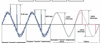
• When choosing a surge protector, it is important to pay attention to the total energy of peak surges of parasitic voltage (in joules), which the device is theoretically able to filter and extinguish at any given time without self-destruction. However, the maximum number of joules in the filter specification is also not the ultimate truth, since a properly designed filter is capable of “grounding” part of the energy through varistors. However, during the selection process, the filter marking in joules should not be discounted.

• The next important parameter is the maximum interference current for which the filter is designed, in amperes. In addition, the surge protector can also be rated according to its maximum load rating, which can be specified in either amps or watts.

• Some manufacturers also add to the list of characteristics of surge protectors the maximum permissible voltage (in volts), the level of attenuation of high-frequency interference for different frequencies (in decibels) and the presence of overload protection - for example, from overheating. Finally, a number of filter parameters that determine its choice in each individual case: cable length, number of sockets, the possibility of wall mounting, the presence of additional filters for telephone lines and twisted pair cables, the presence of USB ports, and so on.

Second order low pass filters

So far we have assumed that an RC low pass filter consists of one resistor and one capacitor. This configuration is a first order filter .

The "order" of a passive filter is determined by the number of reactive elements, that is, capacitors or inductors, that are present in the circuit. A higher order filter has more reactive elements, which results in a larger phase shift and a steeper frequency response rolloff. This second characteristic is the main reason for increasing the filter order.

By adding one reactive element to the filter, for example going from first to second order or from second to third order, we increase the maximum roll-off by 20 dB/decade. A steeper roll-off results in a faster transition from low attenuation to high attenuation, and this can lead to improved performance when there is no wide bandwidth separating the necessary frequency components from the noise components.

Second-order filters are usually built around a resonant circuit consisting of an inductor and a capacitor (this topology is called "RLC", i.e. resistor-inductor-capacitor). However, it is also possible to create second-order RC filters. As shown in the figure below, all we need to do is cascade two first order RC filters.

Figure 12 – Second order RC low pass filter

While this topology certainly produces a second-order response, it is not widely used—as we will see in the next section, its frequency response is often inferior to that of a second-order active filter or a second-order RLC filter.

Electrical filters

In addition to the above, power supply filters are installed in any equipment. Their task is to pass only a voltage with a frequency of 50 Hz inside, and filter out the rest. The equipment produced in the USSR was not capable of boasting high-quality filtration; the requirements were different. Today, sensitive electronics are easily damaged by static and normal interference. The interference easily burned out the graphics adapters of the first computers.

Gradually, electronics have become more secure, but a surge protector is included in any equipment that contains microcircuits. This is not entirely correct; running engines of any type create a lot of interference:

• Asynchronous ones create large voltage surges during start-up and start-up. During operation, the influence on the supply circuit is not so great.
• Collectors constantly clog the power line with interference due to sparking. A running vacuum cleaner greatly disturbs the neighbors.

Filters for control and protective equipment

In addition to electrical filters for power supply circuits of household equipment, unique equipment with similar tasks is found in industry. We are now talking about regulation. During the operation of engines, interference is created, special filters deal with this situation, but efficiency is a separate line. This includes the power factor and the reactive component.

When the engine is running, it sometimes happens that energy is transferred back to the network. For example, during dynamic braking, the shaft briefly enters the generation zone, and the power circuit receives a voltage surge. But even in nominal modes the process of power return develops.

Substation transformers do not generate voltage for return. The presence of reactance in the circuit leads to this. Something like an oscillatory circuit is formed, along which energy scurries idlely back and forth. Warms up the wires without doing any useful work. This has long been noticed; sometimes the enterprise is fined. Power engineers require the installation of reactive (returned) power meters.

To analyze industrial circuits, the method of symmetrical components was developed in 1918. It turned out that the current consumed is represented in the form of three components:

1. Direct sequence.
2. Reverse sequence.
3. Zero sequence.

In literature, especially modern literature, there is no clear description of the meaning of expressions. Deliberately creating confusion only dulls readers. In fact, the names clearly define the subject of the conversation, accurately reflecting the essence. Positive sequence is present with purely active power, when energy is not reflected back, and zero sequence shows whether currents flow in the neutral circuit. The latter happens in case of accidents or unbalanced load. The opposite in meaning characterizes reactive power and occurs under identical conditions.

Symmetrical components

Due to the presence of reactances along three-phase current lines, the voltage is asymmetrical. It is deviated from the nominal value by a certain angle in the vector diagram. As a result, analysis becomes difficult. Current flows simultaneously to power the equipment and back - reflected by the reactive part of the resistance.

Analysis using the method of symmetrical components was invented. Where each signal is decomposed into sequences, as indicated above. Any unsymmetrical voltage or current is represented as the sum of three symmetrical components. Each characterizes a specific process. For example, positive sequence characterizes power consumption. The vector addition of all three gives the voltage or current in the phase in which they flow through the circuit.

In direct sequence, the vectors are shifted in adjacent lines by 120 degrees, forming a supply transformer. In reverse it is similar, but the order of the phases is reversed. If we take direct order, the phase shift is 240 degrees. This is the reason for the name reverse sequence. The third row of vectors is fundamentally different from the other two. In it, the phase shift between voltages or currents is zero. They rotate synchronously.

To carry out these mathematical operations, special formulas have been created. The result of decomposition of an asymmetric sequence is shown in the figure. Since the method is artificial, the components cannot be seen using conventional ammeters and voltmeters. The ideal cases are exceptions:

1. In ideally symmetrical consumption modes across all phases or similar short circuits, we see a direct sequence on the oscilloscope.
2. A reverse sequence is observed in the event of a short circuit in one or two phases. Or in the case of pronounced asymmetry of consumption.
3. The same is said about the zero sequence. In case of short circuits between phases, such a component is absent. And it manifests itself clearly only in case of leaks on the ground.

So, any three-phase network is represented by three fictitious ones, where the listed sequences flow separately. And the values ​​of currents and voltages can then be used for regulation and protection. To implement this in practice, symmetrical sequence relay filters are used.

Balanced component filters

Balanced component filters work with voltage or current and are connected through appropriate transformers. The input measured values ​​are received at the input of these devices, and a control signal is generated at the output. The voltage is usually selected according to a star circuit; it is necessary to obtain information for each line separately.

Sequence filters are considered specific equipment and are so named because they do not produce control actions in the absence of a target signal. Even if there are parameters at the input. It turns out that they perform a filtering function. Hence the requirement for three types. For example, positive sequence filters are used to take into account active energy. But in most cases, the equipment becomes part of the equipment of large enterprises.

There are combined filters. All types of short circuits are not tracked by one type of sequence. Symmetrical sequence filters are included in relays that are not capable of working with conventional, commercially produced ones. When trying to adjust their load characteristics, the volume increases greatly and the mass increases. This is the secret of the strange name - filter relay.

An additional feature is the absence of a single body. The filter components are located separately due to the presence of heterogeneous devices in the composition: transformers, chokes, capacitors, resistors, etc. In addition to current and voltage, these devices are also capable of monitoring power. In the latter case, it becomes possible to implement counters based on them. But, as mentioned above, electrical filter relays are much more often used in protection circuits.

Amplitude-frequency response of a second-order RC filter

We can try to create a second order RC low pass filter by designing the first order filter according to the required cutoff frequency and then connecting these two first order stages in series. This will produce a filter that has a similar overall frequency response and a maximum roll-off of 40 dB/decade instead of 20 dB/decade.

However, if we look at the frequency response more closely, we will see that the frequency has decreased by -3 dB. The second order RC filter does not behave as expected because the two links are not independent - we cannot simply connect the two links together and analyze the circuit as a first order low pass filter followed by an identical first order low pass filter.

Moreover, even if we insert a buffer between these two links so that the first RC link and the second RC link can act as independent filters, the attenuation at the original cutoff frequency will be 6 dB instead of 3 dB. This is precisely because the two stages operate independently - the first filter introduces 3 dB of attenuation at the cutoff frequency, and the second filter adds another 3 dB of attenuation.

Figure 13 – Comparison of amplitude-frequency characteristics of second-order low-pass filters

The main limitation of a second-order RC low-pass filter is that the designer cannot fine-tune the transition from passband to stopband by adjusting the quality factor (Q) of the filter; This parameter indicates how smooth the amplitude-frequency response is. If you cascade two identical RC low pass filters, the overall transfer function is the same as the second order response, but the quality factor is always 0.5. When Q = 0.5, the filter is on the verge of excessive attenuation, and this results in a frequency response that sags in the transition region. Second-order active filters and second-order resonant filters do not have this limitation; the designer can control the quality factor and thus fine-tune the amplitude-frequency response in the transition region.

Complex filters

What happens if you connect two first-order filters one after the other? Oddly enough, this will result in a second order filter.

Its frequency response will be steeper, namely 12 dB/octave, which is typical for second-order filters. Can you guess what the slope of the third order filter will be ? That's right, add 6 dB/octave and get 18 dB/octave. Accordingly, for a 4th order filter the frequency response slope will already be 24 dB/octave, etc. That is, the more links we connect, the steeper the slope of the frequency response will be and the better the filter characteristics will be. This is all true, but you forgot that each subsequent stage contributes to the weakening of the signal.

In the above diagrams, we built the frequency response of the filter without the internal resistance of the generator and also without a load. That is, in this case, the resistance at the filter output is infinity. This means that it is advisable to make sure that each subsequent stage has a significantly higher input impedance than the previous one. Currently, cascading links have already sunk into oblivion and now they use active filters that are built on op-amps.

Summary

• All electrical signals contain a mixture of desired frequency components and unwanted frequency components. Unwanted frequency components are typically caused by noise and interference, and in some situations they will negatively impact system performance.
• A filter is a circuit that responds differently to different parts of the signal spectrum. A low-pass filter is designed to pass low-frequency components and block high-frequency components.
• The cutoff frequency of a low-pass filter indicates the frequency region in which the filter transitions from low attenuation to significant attenuation.
• The output voltage of an RC low-pass filter can be calculated by considering the circuit as a voltage divider consisting of a (frequency-independent) resistive resistance and a (frequency-dependent) reactance.
• Plotting output amplitude (in dB on the vertical axis) versus frequency (in hertz on a logarithmic scale on the horizontal axis) is a convenient and effective way to test the theoretical behavior of a filter (frequency response). You can also use a graph of output signal phase versus frequency on a logarithmic scale to determine the amount of phase shift that will be applied to the input signal (phase-frequency response).
• The second-order filter provides a steeper rolloff; this second-order characteristic is useful when the signal does not provide a wide separation bandwidth between the desired frequency components and the unwanted frequency components.
• You can create a second order RC low pass filter by creating two identical first order RC low pass filters and then connecting the output of one to the input of the other. The resulting frequency -3 dB will be lower than expected.

Original article:

• Robert Keim. What Is a Low Pass Filter? A Tutorial on the Basics of Passive RC Filters

Order

Filter order describes the degree to which frequencies above or below the corresponding cutoff frequency are accepted or rejected. A first order filter whose cutoff frequency is (F) will present an attenuation of 6 in the first octave (2F), 12 dB in the second octave (4F), 18 dB in the third octave (8F) and so on. If we want to know the slope of a filter's attenuation when we have a frequency ratio expressed in decades (10F), the fit would be 20 dB/decade for first order, 40 dB for second, etc. (always displayed on a logarithmic scale).

To implement higher order analog filters, it is common to connect 1st or 2nd order filters in series, because the higher the order, the more complex the filter. However, in the case of digital filters, this typically results in more than 100 orders of magnitude.