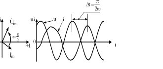
Rationale for vector diagram
Let us assume that the current is given by the equation
i = Imsin(ωt +Ψ)
Let us draw two mutually perpendicular axes and from the point of intersection of the axes we draw a vector Im , the length of which on a certain scale Mi expresses the amplitude of the current Im :
Im = Im/Mi
We choose the direction of the vector so that with the positive direction of the horizontal axis the vector makes an angle equal to the initial phase Ψ (Fig. 12.10).
The projection of this vector onto the vertical axis determines the instantaneous current at the initial time: i0 = ImsinΨ .
Let's imagine that the vector Im rotates counterclockwise with an angular velocity equal to the angular frequency ω . Its position at any time is determined by the angle ωt + Ψ ,
Then the instantaneous current for an arbitrary moment of time t can be determined by the projection of the vector Im onto the vertical axis at this moment of time.
Next article addition and subtraction of vectors in a vector diagram.
For example, for t = t1
i1 = Imsin(ωt1 +Ψ)
in general
i = Imsin(ωt +Ψ)
We obtained the same equation as the alternating current was specified, which indicates the possibility of depicting the current as a rotating vector when applied to the drawing in the initial position.
Alternating current. Vector diagrams
Alternating current is a current that changes both in magnitude and direction over time. In electrical engineering, sinusoidal alternating current is mainly used, i.e. changing over time according to the law of sine. Mathematically, the instantaneous value of the sinusoidal current is expressed as follows:
, (2.1)
where i
– instantaneous current value at time
t
,
Im
– maximum (amplitude) current value,
ω
– circular (angular) frequency.
The angular frequency ω
is related to the frequency
f
of the alternating current by the expression .
The expression ω t
is called the oscillation phase or phase angle.
The phase characterizes the state of the current change process at a given time t
.
The sinusoidal current graph is shown in Fig. 2.1a. The ordinate axis shows the instantaneous current value, and the abscissa axis shows the phase angle in degrees or radians. t can also be plotted on the x-axis
, and not the value
ω t
, and it is convenient to measure time in fractions of the
period T.
Rice. 2.1. Image of sinusoidal current graph (a)
and vector diagram (b)
In addition to the graphical and trigonometric representation of sinusoidal current, there is also a method of rotating radius vector (Fig. 2.1 b). When analyzing alternating current parameters, this method in a number of cases facilitates the derivation of certain formulas, and is also very visual in a qualitative examination of the processes occurring in alternating current circuits. Let's imagine the maximum current Im
as a vector
I on some arbitrary scale. Now suppose that this vector rotates around its origin - point 0 counterclockwise with an angular velocity ω
equal to the angular frequency
ω
.
Let at time t = 0
vector
I coincides in direction with the OX axis (initial axis). Then by the time t = t 1
the vector will rotate through an angle
ω t 1
relative to the initial axis.
The projection of vector I in this position onto the vertical axis is equal to the segment OA:
. (2.2)
Comparing formulas (2.1) and (2.2) you can see that the segment OA on the selected scale gives the instantaneous value of the current at time t = t 1
, if at time
t = 0
the instantaneous value of this sinusoidal current was equal to zero (projection of vector
I onto the vertical axis at the initial moment t = 0
).
Thus, we can assume that the projection of the rotating radius vector I onto the vertical axis at any moment of time represents, on a certain scale, the instantaneous value of the current at that moment. In the same way, you can construct a detailed graphical dependence of this quantity on time. In Fig. Figure 2.2 shows the vector I representing a variable and the corresponding expanded vector diagram for i
.
Rice. 2.2. Graphical and vector representation of sinusoidal current
If at the initial time t = 0
vector
I makes a certain angle with the initial axis, then the expanded diagram for this case is presented in Fig. 2.3 a and 2.3 b. The instantaneous value of the current depending on time in these cases is written as follows: for Fig. 2.3 a, and for Fig. 2.3 b. The angle that determines the position of vector I at time t = 0
is called the initial phase.
Rice. 2.3 Graphic and vector representation of vector I
for two initial phases
If two periodic quantities in their measurements simultaneously pass through zero and maximum values, simultaneously increase and decrease, then these quantities can be said to be in phase. In Fig. Figure 2.4 shows the curves: current and voltage, coinciding in phase, obtained by rotating two vectors U and I , coinciding in direction and having an initial phase equal to 0. In Fig. 2.5 shows two U
and
I
, having different initial phases.
Rice. 2.4. Trigonometric image and vector diagram
for the case of voltage and current being in phase
Initial phase difference φ = α – β
called phase shift. In Fig. 2.5 it can be seen that the current curve is ahead of the voltage curve in phase, because it reaches its maximum value earlier, begins to decrease earlier, etc. It is worth noting that when these two vectors are rotated, the angle between them does not change.
Rice. 2.5. Display of U
and
I
, having different
initial phases in vector and graphical form
With the simultaneous action of two or more variable homogeneous quantities (in particular, two currents or two voltages), the instantaneous values of these quantities are added. The result of such addition can be depicted graphically by constructing two sinusoids, and at each moment of time adding the ordinates of these sinusoids and using the sum of the ordinates to construct a third sinusoid. At the same time, it is much simpler and more visual to use the method of geometric addition of radius vectors representing the corresponding quantities. In this case, it is possible to determine not only the amplitude value, but also the initial phase. In Fig. Figure 2.6 shows the addition of two currents I 1
and
I 2
with different amplitude values and different phases.
Rice. 2.6. Addition of two sinusoidal currents by vector
and graphically
It is worth noting that, as a rule, it is important to know not the instantaneous value of current or voltage, but to be able to evaluate the effect of alternating current over a certain period of time, i.e. know some average value of alternating current or voltage. Depending on the type of current action (chemical, thermal, electrodynamic, etc.), different averaging should be used. For example, to evaluate a chemical effect, one should take the arithmetic average of the alternating current over a certain period of time. For sinusoidal alternating current, this value is zero per period. Therefore, the use of alternating current for the electrolysis process is not suitable. In turn, the thermal and electrodynamic effect of the current is proportional to the square of the current strength and. therefore, the rms value of the alternating current is of interest in these cases. Let us calculate the root mean square value of the current using the example of the thermal effect of current. In the case of alternating current in a substance for an infinitely small period of time dt
the amount of heat
dQ
, i.e.: , where
i
is the instantaneous value of the alternating current during the time
dt.
The amount of heat over a period of time
T
is equal to:
. (2.3)
Next, we find the value of direct current I
for the same period of time
T
, during which an equivalent amount of heat
Q will be released.
Since, then.
Now let's substitute expression (2.3) instead of Q
: . The AC value that acts similar to the DC value is called the AC rms value. Mathematically, this sentence can be written as follows:
. (2.4)
From the last expression it is clear that the effective value of the current I
equal to the rms value of the alternating current.
Let us obtain the relationship between the effective value of the current I and the amplitude value of the current Im for an alternating sinusoidal current. To do this, determine the value of the integral:
.
It can be seen that: the first integral is: , the second integral is . Therefore, for the case of sinusoidal current we can write:
. (2.5)
The relationship between the effective and amplitude values of alternating voltage looks similar:
. (2.6)
It is worth noting that electrical measuring instruments (ammeters and voltmeters) of electromagnetic, electrodynamic and some other systems show the rms value of current and voltage, and therefore, the effective value of these quantities. In turn, the devices of the magnetoelectric system show the arithmetic mean or simply the average value of the alternating current. For this reason, the instruments of this system are not suitable for measuring alternating current parameters.
Let us now consider electrical circuits containing various types of load, in particular active resistance (resistor), inductive reactance (inductor), capacitive reactance (capacitor).
1) AC circuit containing active resistance
.
Let to the active resistance R
AC voltage is applied.
Then an alternating current i
of the same frequency will flow through the circuit, but in phase the current, generally speaking, may not be in phase with the voltage, i.e. the expression for the instantaneous current value is:
. (2.7)
For infinitesimal periods of time, we have the right to apply Ohm’s law to alternating current, which is valid for direct current, assuming that currents and voltages will not change in these short periods of time. For instantaneous values of current and voltage, we can write:
. (2.8)
Replacing U
in expression (2.8) we get:
. (2.9)
Comparing expressions (2.7) and (2.9) one can see that , and φ
= 0. Consequently, the phases of the current and voltage are the same, the phase difference is zero, i.e. current and voltage are in phase. The electrical circuit and the vector diagram for it are shown in Fig. 2.7.
Fig.2.7. An electrical circuit containing active resistance (a),
and a vector diagram for it (b)
2) An alternating current circuit containing inductive reactance.
In Fig. Figure 2.8 shows an alternating current circuit containing an inductor. For simplicity of reasoning, we will consider this inductor to be ideal, i.e. its active resistance is zero. In practice, especially in the high-frequency region, this assumption is correct.
Rice. 2.8. AC circuit containing an inductor
Let us apply an alternating voltage to this coil. In this case, an alternating current will flow through the coil, which, with its magnetic field, will induce a variable self-inductive emf E in the coil
.
According to Kirchhoff’s law, for instantaneous values of alternating current we have, but since R
= 0, then
U = -
E. In turn, from the law of electromagnetic induction it is known that:
, (2.10)
where L
– coefficient of self-inductance of the coil, or simply inductance. Because The current may not be in phase with the voltage, let's present it in the form:
, (2.11)
where φ
– phase shift between current and voltage. Substituting (2.11) into (2.10) and differentiating, we can obtain:
. (2.12)
Comparing (2.9) and (2.12), we can write:
. (2.13)
From this we can draw the following conclusions:
A) . Since the value ωL
has the same dimension as the resistance; by analogy with Ohm’s law
U = IR
for active resistance, the product
ωL
the inductive reactance of the coil. The presence of inductive reactance in the circuit is due to the counteraction of the self-inductive emf E to the alternating current flowing in the circuit according to Lenz’s rule. Inductive reactance, as well as self-inductive emf, depends on the inductance of the circuit and the rate of change of current, which in the case of alternating current is determined by the frequency of the current.
b) if φ =
-90º.
Therefore, in the expression for current (2.11), the angle φ
should be replaced by an angle of 90º. Thus we can write:
(2.14)
From this expression we can conclude that the current in the inductor is out of phase with the voltage applied to the coil by an angle of 90º. In Fig. Figure 2.9 shows a graphical and vector view of current and voltage for the case of an ideal inductor.
Rice. 2.9. Vector and graphical representation of current and voltage
AC circuit containing inductive reactance
At the same time, in some cases, consider the active resistance R
coils cannot be equal to zero.
In this case, the inductor is considered as a series connection of active resistance R
and pure inductance
L
without active resistance, and the resulting RL circuit is analyzed (Fig. 2.10).
Relationships obtained for the amplitude values of the current Im
and voltages
Um
are
also valid for the effective values of current
I
and voltage
U. In particular, if we divide both sides of the equality by √2, we get the relation . Similarly, one can obtain an expression for active resistance, i.e. . I
flows through the circuit (Fig. 2.10) , then the voltage across the active resistance is
Ua = IR
, and across the inductive
UL = IXL
.
Rice. 2.10. Electrical circuit illustrating an inductor
with non-zero active resistance
Let's construct a vector diagram of voltages for this circuit, but instead of amplitude values we will use effective voltage values, which is equivalent to changing the scale of the segments by √2 times. Let us set aside the vector Ua = IR
in the direction of current
I
, and vector
UL
directed relative to I at 90º counterclockwise (Fig. 2.11).
The total voltage is equal to the vector sum of voltages Ua
and
UL
.
Rice. 2.11. Vector and graphical representation of stresses
in RL circuit
Using the vector addition rule, the expression for the total voltage can be written as follows:
(2.15)
From this expression it is clear that the phase shift between the total voltage and current depends on the ratio Ua
and
UL
, and therefore also on the ratio of
R
and
XL
.
From Fig. 2.11 it is clear that . By dividing the full expression by the current value I
, we can find the total resistance
Zk
of the coil, equal to:
(2.16)
In turn, for the phase shift the following expression can be written:
(2.17)
3) An alternating current circuit containing a capacitor.
If the plates of a capacitor are connected to a direct current source, then the current will flow in the circuit until a potential difference equal to the emf of the source arises on the plates of the capacitor due to the flowing charge. If an alternating voltage is applied to the capacitor, then the capacitor will be continuously recharged, and alternating current will flow in the circuit all the time, and the larger the capacitor’s capacitance, the greater the current will flow through the circuit (Fig. 2.12, 2.13).
Rice. 2.12. AC circuit containing a capacitor
Rice. 2.13. Vector and graphical representation of current and voltage
in a circuit containing a capacitor
Let an alternating voltage be applied to the capacitor, in this case the charge of the capacitor will change over time in the same way as the voltage on it changes. If C
is the capacitance of the capacitor, then .
Over an infinitesimal period of time dt,
the charge changes by the amount
dq
. Knowing the definition of current, we can write: . Having accepted, you can write: . Since it has the dimension of resistance, it is therefore designated and called capacitive reactance. From the formulas for current and voltage it is clear that current leads voltage by 90°.
Let us now consider an alternating current circuit consisting of series-connected resistances R
, capacitor
C
and ideal inductor
L
(Fig. 2.14).
Since the elements in the circuit are connected in series, the same current I
. Consequently, the voltage on the circuit elements is determined according to Ohm’s law for a section of the circuit: , , .
Rice. 2.14. An alternating current circuit containing a resistor, capacitor and inductor connected in series
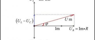
Let's construct a vector diagram for such a circuit. Let us take the initial phase of the current equal to 0, i.e. vector I will be directed along the initial axis. The voltage Ua should be set aside in the same direction, because the current and voltage across the active resistance are in phase. The voltage across the inductor UL will lead the current by 90º, and the voltage across the capacitor UC will lag the current by 90º. The voltage triangle for circuit (2.14) is shown in Fig. 2.15.
Rice. 2.15. Vector diagram for a circuit in which in series
connected resistance, capacitor and inductor
The total voltage of the circuit is equal to the geometric sum of the voltages in individual sections. In order to find it, you must first add the opposite vectors UL and UC , and then add the vector Ua . The vector sum UL + UC is equal to the algebraic difference of the modules of the vectors UL
and
UC
, i.e.
(UL - UC)
. Then:
. (2.18)
Substituting in (2.18) instead of Ua
,
UL
and
UC
their expressions through the current
I
and the corresponding resistances can be obtained:
.
Let's denote the expression by Z:
. (2.19)
Z value
is called the impedance of the circuit.
From this expression it can be seen that the total resistance of the circuit is calculated through R
,
XL
,
XC
in the same way as the total voltage of the entire circuit is calculated through the voltages on the circuit components. By analogy with Fig. 2.15 you can build a resistance triangle (Fig. 2.16).
Rice. 2.16. Resistance triangle for a complete circuit
alternating current
Phase shift φ
between the current
I
and the total voltage
U
is determined from the relations:
; , (2.20)
Sign of the phase shift φ
depends on the predominance of inductive or capacitive load in the circuit.
Let's consider the case when the inductive reactance is equal to the capacitive reactance in the alternating current circuit, i.e. . Then . Consequently, φ =
0, i.e.
there is no phase shift between current and voltage, and total resistance Z =
R.
In this case, they speak of the presence of voltage resonance in the circuit. The phenomenon of resonance is used in radio engineering to isolate the signal of a particular radio station. In turn, in electrical engineering, as a rule, voltage resonance is a dangerous phenomenon, because it is associated with the occurrence of overvoltages on circuit elements that are several times higher than the operating voltage of the installation. At the same time, fuses and similar fuses are not capable of protecting the installation from these overvoltages. Let's look at an example. There is an alternating current circuit in which an active resistance R =
10 Ohms and reactance
XL = XC =
1000 Ohms are connected in series.
Let us take the applied voltage equal to U =
100 V. Then the current in the circuit is .
Then the voltages on the inductor and on the capacitor will be respectively equal to UL = IXL =
10
A ·
1000
О
=10000
V
and
UC = IXC =
10
А ·
1000
Ohm
=
10000 V. It can be seen that the voltages on the circuit elements are many times higher than the source voltage. If the insulation in the capacitor and/or inductor is not designed to withstand this voltage, then these circuit elements will fail.
In general, the voltage across the inductor or capacitor at resonance is as many times as the voltage supplied to the entire circuit as the reactance XL
and
XC
is more active resistance
R
:
; . (2.21)
Thus, overvoltage at resonance occurs at R < XL
and
R < XC
. Since resonance occurs under the condition , it is easy to obtain an expression for the resonant frequency, namely:
. (2.22)
Substituting (2.22) into expression XL
and
XC
, we can obtain the general condition for the occurrence of overvoltage at resonance:
; ; . (2.23)
The value does not depend on frequency and is an intrinsic characteristic of the circuit. Since this quantity has the dimension of resistance, it is called the characteristic or characteristic impedance of the circuit ρ
.
It is worth noting that the voltage across the capacitor UC
and inductor
UL
will not always be maximum at resonance.
The phenomenon of resonance in a circuit can be achieved by selecting either the frequency ω
, or the capacitance of the capacitor
C
,
or the inductance of the coil
L. A graph of UC
and
UL
versus frequency is shown in Fig.
2.17.
be
seen that the voltage UC
and
UL
are reached at different frequencies
ω C
and
ω L. One of them is less and the other is greater than the resonant frequency ω0
.
The lower the active resistance of the circuit, the higher and closer the maximums UL
and
UC
are to each other.
They coincide at R = 0
, and, conversely, with a sufficiently large resistance
R
(
R >ρ
), the dependences
UC (ω)
and
UL (ω)
do not have maxima.
Rice. 2.17. Frequency dependencies UC
,
UL
and
I
Rice. 2.18. Capacitive dependences UC
,
UL
and
I
In this laboratory work, the circuit is tuned to resonance by changing the capacitance C
.
The dependences UC (C)
and
UL (C)
are shown in Fig.
2.18. At resonant capacitance, the voltage across the inductor reaches its maximum. In turn, the voltage on the capacitor UC
reaches a maximum at a capacitance less than
C res
.
In the practical implementation of the voltage resonance mode, the presence of active resistance in the inductor should be taken into account. A voltmeter connected to the coil shows the total voltage across it, which corresponds to . This voltage at resonance is not equal to the voltage across the capacitor UC
.
Consequently, tuning for resonance is carried out at the maximum
current I.
Let us now consider the power released in the alternating current circuit. Since current and voltage change, then, accordingly, the power in an alternating current circuit is a variable quantity, and, therefore, we can only talk about instantaneous power p
, determined by the product of the instantaneous current value and the instantaneous voltage value, i.e.
p = i u
.
In general, when the phase difference between current and voltage is φ
, the instantaneous power
p
will be determined by the following expression:
. (2.24)
By applying a series of trigonometric transformations, we can obtain:
. (2.25)
Replacing the amplitude values of current and voltage with actual values, we obtain:
. (2.26)
The last expression is a constant component and a harmonic component varying with double frequency 2ω t
.
In the case of an active load ( φ =
0, cos
φ =
1), the instantaneous power is determined by the expression.
In the case of a purely inductive load ( φ =
90°, cos
φ =
0), the instantaneous power is given by: In the case of a purely capacitive load, the expression for instantaneous power differs from the previous one only in sign, i.e. . The presence of this sign is clearly manifested during resonance. Graphs for instantaneous powers for the case of active, inductive and capacitive loads are shown in Fig. 2.19 (a, b, c).
Rice. 2.19 a. Frequency dependence of instantaneous power
in case of active load
Rice. 2.19 b. Frequency dependence of instantaneous power
in case of inductive load
Rice. 2.19 c. Frequency dependence of instantaneous power
in case of capacitive load
In practice, it is not the instantaneous value of power that is of interest, but its average value over a long period of time, corresponding to a large number of periods of power fluctuations. This power can be measured using a wattmeter. Since the wattmeter needle does not have time to track instantaneous power values, it is set in a position corresponding to a certain average power value. Let's determine this value. AC operation dA
over a short period of time
dt
is equal to . In turn, the work per period is equal to , the average power p for the same time is equal to . Next, taking into account formula (2.26), we can write:
,
or
.
The second integral is equal to zero, because the integral of the cosine function over the entire period is equal to zero. Therefore, the average power has the form:
, (2.27)
those. determined not only by the effective values of current and voltage at the consumer, but also by the phase shift φ
between current and voltage.
The value of cos φ
is called the power factor, and it plays a significant role among the parameters characterizing the consumer.
The smaller cos φ
, the less efficiently the power supplied from the generator to the consumer is used and the greater the energy loss in the supplied wires.
Since in the general case, the expression for the average power can be written in the form. Next, replacing the ratio of the effective voltage to the total resistance through the current, we have. Thus, the average power in an alternating current circuit is equal to the power allocated to the active resistance R
chains.
Active power P
is the main quantity characterizing energy processes in alternating current circuits, but not the only one.
For example, in the case of a purely inductive load, the active power is zero. However, in this case, alternating current flows through the supply wires and energy is exchanged between the generator and the consumer (signs + and – in Fig. 2.19 b.) The intensity of this exchange depends on the effective values of the current
I
and
voltage
U
and is determined by the reactive power
Q. A similar energy exchange occurs with a purely capacitive load (Fig. 2.19 c). For this reason, inductive and capacitive loads are generally called reactive. In the case of a mixed load, for example, active-inductive, reactive power is determined by the expression. Since in this case the energy processes in the circuit will be determined by both active power P
and reactive power
Q
S
was introduced . The total power in the circuit for any type of load is equal to the product of the effective current value and the effective voltage value, i.e. .Using a voltage vector diagram for a load, you can obtain the relationship between the total, active and reactive powers for this load. To do this, we multiply the sides of the voltage vector diagram by the current and get a power triangle (Fig. 2.20). From this triangle we can write the following expression for the total power: . The unit of measurement for active power is watt (W) or kilowatt (kW), reactive power is volt-ampere reactive (Var) or kilovolt-ampere reactive (kVar), apparent power is volt-ampere (VA) or kilovolt-ampere (kVA) . Such a difference in the name, in addition to the numerical value of the power, shows what kind of power we are talking about.
Rice. 2.20. AC Circuit Power Triangle
Practical part
Task I: Study of an unbranched alternating current circuit.
1) Assemble the electrical circuit shown in Fig. 2.21.
Devices and components:
a wattmeter with a current measurement limit of 1 - 2 A, an ammeter with a measurement limit of 0.25 - 1 A, two voltmeters with a measurement limit of 75 V (the second voltmeter is used to measure voltages in different sections of the circuit), a single-phase transformer coil for 220 V or an inductor for 1200 turns (coil core open), capacitor magazine. A constant capacitor of 10 μF should be connected in parallel to the capacitor magazine.
Note:
For the convenience of measurements, the second voltmeter should be connected in parallel to the volt winding of the wattmeter and then free conductors should be removed from this voltmeter to be able to connect this measuring system to various sections of the circuit.
Rice. 2.21. Working electrical circuit for task I
Table 2.1
| Mode | Chain section | Measure | Calculate | ||||||||
| I,A | U,V | P, W | Z, Ohm | R, Ohm | XL,Ohm | XC,Ohm | S, Va | Q, Var | cosφ | ||
| XL>XC C = 40 µF | R | ||||||||||
| L | |||||||||||
| C | |||||||||||
| R+L+C | |||||||||||
| XL=XC C ≈ 20uF | R | ||||||||||
| L | |||||||||||
| C | |||||||||||
| R+L+C | |||||||||||
| XL < XC C = 10 µF | R | ||||||||||
| L | |||||||||||
| C | |||||||||||
| R+L+C | |||||||||||
2) For three different values of capacitor capacitance (see Table 2.1), measure current, voltage and active power (wattmeter measures active power) on active resistance (R1 + R3), on inductive reactance L, capacitive reactance C, as well as on all section of the chain, i.e. R + L + C. The source voltage should be set to about 70 V. The resulting data should be entered into table 2.1.
Note:
In experiment 2 (
XL = XC
), achieve voltage resonance, focusing on the highest current in the circuit.
3) Make calculations according to table 2.1.
4) Construct scaled vector diagrams of voltages, triangles of resistance and power for all three experiments, taking into account that the voltmeter connected to the inductor shows the total voltage in this area, and not the purely inductive component.
Task II: Study of the phenomenon of voltage resonance.
1) Assemble the circuit shown in Fig. 2.22.
Note:
On the left in the above diagram there is a three-phase transformer. In this circuit, the windings of this transformer are connected as a star, i.e. three-phase voltage is supplied to the beginning of the primary winding (A, B, C) (from terminals A, B, C) from the stand, the ends of the primary winding X, Y, Z are connected to each other, the ends of the secondary winding x, y, z are also connected to each other , three-phase voltage is removed from terminals a, b, c. When performing this task, any two of these terminals are used as a voltage source.
Rice. 2.22. Working electrical circuit for task II
Devices and components:
an ammeter with a measurement limit of 0.25 - 1 A, a voltmeter V1 with a measurement limit of up to 60 V (use 15 V), two voltmeters (V2 and V3) with a measurement limit of 75 V, a single-phase transformer coil of 220 V or an inductor of 1200 turns (core coils are open), capacitor magazine.
2) Make calculations according to table 2.2.
Table 2.2
| Measure | Calculate | |||||||||
| C, µF | U, V | UL, V | UC, V | I, A | Z, Ohm | Zk, Ohm | XL, Ohm | XC, Ohm | S, Va | cosφ |
| 10 | ||||||||||
| 12 | ||||||||||
| 14 | ||||||||||
| 15 | ||||||||||
| 16 | ||||||||||
| 17 | ||||||||||
| 18 | ||||||||||
| 19 | ||||||||||
| 20 | ||||||||||
| 21 | ||||||||||
| 22 | ||||||||||
| 23 | ||||||||||
| 24 | ||||||||||
| 26 | ||||||||||
| 28 | ||||||||||
| 30 | ||||||||||
| 32 | ||||||||||
3) Based on measurement and calculation data, construct dependency graphs in the general picture: I = f ( C )
,
UC = f ( C )
,
UL = f ( C )
,
Z = f ( C )
, cos
φ = f ( C )
.
Control questions
1) What parameters characterize sinusoidal current and voltage?
2) What is the relationship between a sinusoidally varying quantity and the vector x representing it? How to make the transition from a sine curve to a vector diagram and vice versa?
3) What is called the root-mean-square (rms) value of the sinusoidal current?
4) What is the relationship between peak and peak value of current?
5) What current value (instantaneous, amplitude, average, effective) is shown by an ammeter connected to an alternating current circuit?
6) Why is the resistance of a coil in an AC circuit greater than its resistance in a DC circuit?
7) Reveal the physical meaning of active resistance.
Explain the physical meaning of inductive reactance.
9) Expand the physical meaning of capacitance.
10) Show that the average power in an AC circuit is equal to the active power.
11) What is active, reactive and apparent power in an alternating current circuit? What are the units of measurement for these quantities?
12) What is voltage resonance?
13) Why, during voltage resonance at the terminals of an inductor and capacitor, can the voltage be greater than the voltage applied to the entire circuit?
14) Prove that the maximum of the curve UC (C)
lies to the left of the maximum of the
UL(C)
.
15) Prove that the maximum of the curve UC ( ω )
lies to the left of the maximum of the
UL(ω)
.
16) Will the voltage resonance in the circuit be disrupted if an active resistance is additionally included in this circuit?
a) In series with XC
and
XL
.
b) Parallel to XC
and
XL
.
c) Parallel to XC
or
XL
.
Construction of a vector diagram
By rotating the vector Im' counterclockwise, in a rectangular coordinate system we will construct a graph of changes in its projection onto the vertical axis within one revolution (one period). We obtain the already known graph of the sinusoidal function corresponding to the given equation.
When constructing vectors, positive angles are counted from the positive direction of the horizontal axis counterclockwise, and negative angles are counted along its movement.
In the process of calculating an electrical circuit, a number of sinusoidal quantities are determined. All of them can be depicted on one drawing using rotating vectors, tied to one pair of mutually perpendicular axes.
A set of vectors depicting in one drawing several sinusoidal quantities of the same frequency at the initial moment of time is called a vector diagram.
For example, voltage and current in an electrical circuit are expressed by the equations:
u = 125 sin(ωt + 30°)
i = 12 sin(ωt - 20°).
The vector diagram of such a circuit is shown in Fig. 12.11. If we choose the voltage and current scales
Mu = 50 V/cm; Mi = 4 A/cm;
That
Um = Um/Mu = 125/50 = 2.5 cm ; Im = Im = im/Mi = 12/4 = 3 cm.
A vector diagram contains vectors of sinusoidal quantities of the same frequency, so they rotate with the same frequency and their relative positions do not change.
The time reference point is chosen arbitrarily, so one of the diagram vectors can be directed arbitrarily; the rest must be positioned taking into account the phase shift relative to the first or previous vector.
Types of vector diagrams and rules for their construction
Definition 1
A vector diagram is a set of vectors on a complex line that corresponds to complex parameters and/or quantities of an electrical circuit.
Vector diagrams can be:
- Chiseled.
- High quality.
The construction of scatter plots is carried out in compliance with the scale of all quantities according to the results of numerical analysis. The main purpose of scatter plots is to check the calculation results. High-quality vector diagrams are constructed taking into account the relationships between complex quantities. The construction of this type of diagrams, as a rule, replaces or precedes calculations. In high-quality vector diagrams, the values of parameters (or quantities) and the image scale are unimportant. The main requirement for them is that all relationships between quantities are displayed correctly. This type of diagram is one of the main tools for analyzing AC circuits.
Are you an expert in this subject area? We invite you to become the author of the Directory Working Conditions
Vector diagrams are divided into circular and linear. In a circular vector diagram, the locus of the moving points of the end of the vector is a circle or semicircle. In linear vector diagrams, the locus of the end points of a vector is a straight line.
Before constructing a phasor diagram, an equivalent circuit, which is equivalent to a circuit diagram of an electrical circuit, is first drawn and analyzed. On this diagram, each element of the electrical circuit must be marked, and the directions of all voltages and currents are plotted. Vector diagrams of currents and voltages should be drawn on a large scale, the choice of which is made based on the largest calculated or measured value of electric current or voltage.
Asymmetrical modes in the simplest characteristic cases (short circuit and no-load) can be analyzed based on the construction of vector diagrams.
Let's consider the phase open and short circuit modes when connecting in a star for three- and four-wire systems. In this case, we will make a comparison with the symmetrical operating mode of the circuit, the phase voltages and currents in which will be basic. For this circuit (see Fig. 1, a) the vector diagram of currents and voltages is shown in Fig. 1b (it is assumed that the load is active-inductive in nature). Here
When phase A of the load breaks, we arrive at the vector diagram in Fig. 2.
In this case
.
When there is a short circuit in phase A (three-wire system), the vector diagram in Fig. 3. It follows from it: ; ; ; ; .
If phase A breaks in a four-wire system (the neutral wire in Fig. 1, a is shown by a dotted line, and the current vector is shown by a dotted line in Fig. 1, b); ; .
A symmetrical three-phase receiver when connected in a triangle and the corresponding vector diagram of voltages and currents are shown in Fig. 4.
Here, using the same method of connecting the generator phases; ; ; ; ; .
If the wire breaks in phase A-B of the load, as can be seen from the diagram in Fig. 5, ; , while the currents themselves and, due to the autonomy of the phase operation mode when connecting the load into a triangle, are the same as in the circuit in Fig. 4, a. Thus, ; ; .
The circuit in the event of a break in the linear wire A-A' and the vector diagram corresponding to this case are shown in Fig. 6.
Here
; ; .
Power in three-phase circuits
The instantaneous power of a three-phase energy source is equal to the sum of the instantaneous powers of its phases:
.
The active power of the generator, defined as the average instantaneous power over the period, is equal to
.
Accordingly, the active power of a three-phase receiver taking into account losses in the resistance of the neutral wire
,
reactive
and full
.
Total active power of a symmetrical three-phase system
| . | (1) |
Taking into account that in the symmetric regime for a star the following relations hold:
and for a triangle -
based on (1) for both phase connection methods we obtain
,
where j is the shift angle between phase voltage and current.
Likewise
Let us now prove the previously stated property of balance between a two-phase Tesla system and a symmetrical three-phase system.
1. Two-phase Tesla system
In accordance with Fig. 7
| (2) |
| . | (3) |
Taking into account (2) and (3)
.
Thus, the total instantaneous power of the phases is a constant value equal to the total active power of the source.
2. Symmetrical three-phase circuit
Then
From here
,
those. and for a symmetrical three-phase circuit the property of balance has been proven.
Power measurement in three-phase circuits
Below we consider practical circuits for connecting wattmeters for measuring power in three-phase circuits.
1. Four-wire system, single-ended mode.
Shown in Fig. 8 circuit is called a three-wattmeter circuit.
The total active power of the circuit is determined as the sum of the readings of three wattmeters
.
2. Four-wire system, symmetrical mode.
If the operating mode of the circuit is symmetrical, then to determine the total active power it is enough to limit yourself to one wattmeter (any), connected according to the diagram in Fig. 8. Then, for example, when the device is turned on in phase A,
| . | (4) |
3. Three-wire system, symmetrical mode.
If there is no access to the neutral point, the latter is created artificially by connecting three additional resistors in a star configuration, as shown in Fig. 9 – diagram of a wattmeter with an artificial neutral point.
In this case, it is necessary to satisfy the condition where is the intrinsic resistance of the wattmeter winding. Then the total active power of the three-phase system is determined according to (4).
4. Three-wire system, symmetrical mode; reactive power measurement.
Using one wattmeter in a symmetrical circuit operating mode, you can measure its reactive power. In this case, the wattmeter connection circuit will look like Fig. 10, a. According to the vector diagram in Fig. 10b power measured by the device
Thus, the total reactive power
5. Three-wire system, single-ended mode.
Shown in Fig. 11 circuit is called a two-wattmeter circuit. In it, the sum of the instrument readings is equal to the total active power of the circuit.
Indeed, the instrument readings in this diagram:
.
Then
In conclusion, we note that if in the circuit in Fig. 11 there is a symmetrical operating mode, then based on the instrument readings it is possible to determine the total reactive power of the circuit
| . | (5) |
Literature
- Fundamentals
of circuit theory: Textbook. for universities / G.V. Zeveke, P.A. Ionkin, A.V. Netushil, S.V. Strakhov. –5th ed., revised. –M.: Energoatomizdat, 1989. -528 p. - Bessonov L.A.
Theoretical foundations of electrical engineering: Electric circuits. Textbook for students of electrical engineering, energy and instrument engineering specialties of universities. –7th ed., revised. and additional –M.: Higher. school, 1978. –528 p.
Test questions and tasks
- A phase loss has occurred in a symmetrical three-wire circuit. What will a voltmeter show when connected between the neutral points of the source and receiver?
- How many times the power in the circuit in Fig. 6, and less power in the circuit in Fig. 4, huh?
- In the circuit in Fig. 10, and the symmetrical load is made up of resistive elements. What will the wattmeter show?
- In the circuit in Fig. 10, and the symmetrical load with phase resistance is connected in a star. Line voltage.
- In the circuit in Fig. 11, the load is served by two identical capacitors with XC = 100 Ohms, connected between linear wires A and B, B and C, respectively. Line voltage.
- Based on the construction of a vector diagram of currents and voltages for the symmetrical operating mode of the circuit in Fig. 11 prove relation (5).
Answer: .
Answer: twice.
Answer: .
Determine the wattmeter reading.
Answer: .
Determine the wattmeter readings.
Answer: .
How to Make a Ray Vector Link Diagram in Excel
First, let's take a look at what we are trying to build and visually estimate the amount of work. Looks interesting? Then read on to find out how to create it.
To create a ray diagram in Excel to visually analyze relationships in a network, we need to first understand its different components.
As you can see, the diagram contains the following parts:
- A set of points, each of which represents one stakeholder - network participants.
- A set of grayish thick solid and thin dotted lines representing all relationships between people. Solid lines are strong connections (for example, friends), dotted lines are weak connections (acquaintances).
- A set of green thick and blue dotted lines representing relationships for a selected specific network group member.
- A slicer for selecting a participant's analysis - like a ray diagram control panel.
- A table with summary statistics of the selected person.