Definition
Root mean square (RMS) is a static measure of a variable. This is useful if the function alternates between positive and negative exponents (sine waves). Here we have the square root of the arithmetic mean of squares. In the case of a set of values n (x1, x2, …., xn), the RMS is determined by the formula:
The corresponding formula for a continuous function f (t) calculated on the interval T1 ≤ t ≤ T2:
RMS current for the function over the entire time:
The rms voltage value during the periodic function is equal to the RMS value of one period.
Light bulb and constant voltage
For experiments we will also need a simple 12 Volt car incandescent lamp
Here are its characteristics: operating voltage U = 12 Volts, power P = 21 Watts.
Therefore, knowing the power and voltage of the lamp, you can find out how much current the light bulb will consume. From the formula P=IU, where I is the current strength, you can find I. This means I=P/U=21/12=1.75 Amperes.
Okay, we've sorted out the light bulb. Let's light it up. To do this, set the operating voltage for our lamp on our power supply
We supply voltage from the power supply to the lamp and voila!
We measure the voltage at the alligator terminals of the power supply using a multimeter. Exactly 12 Volts, as expected.
We connect our oscilloscope to the same terminals
Let's look at the oscillogram:
Do you see a straight line? This is a DC voltage oscillogram. Over time, our tension remains the same as it was and does not change. If you do the math, you can figure out what the voltage is. Since one cell has 5 Volts (pictured below left), this means our voltage is 12 Volts. I also plotted this value on the oscilloscope display in the very bottom left corner: 12.03 Volts. That's right.
We measure the current strength. You can learn how to correctly measure the current in a circuit by reading the article How to measure current and voltage with a multimeter?
We got 1.72 Amperes. And as you remember, our calculated value was 1.75 Amps. I think the blame can be shifted to the error of the device or to the light bulb
Application to voltage and current
Let's take a look at a sinusoidally varying voltage:
(a) – Constant voltage and current remain stable. (b) – Graph of voltage and current versus time for 60 Hz AC power. The voltage and current are sinusoidal and in phase for a simple resistance circuit. Frequencies and peak voltages vary greatly
V = V0sin (2πft), where V is the voltage at an instant, V0 is the peak voltage, f is the frequency in Hz. For this simple resistance circuit, I = V/R, so the AC current looks like:
I = I0sin (2πft), where I is the current at an instant and I0 = V0/R is the peak current. Now, using the above definition, we derive the rms voltage and current. First of all we have
Here we have replaced 2πf with ω. Since V0 is a constant, we can expand it by its square root and use the trigonometric formula to replace the square of the sine function.
Integrating what was written:
Since the interval represents an integer number of complete cycles, the terms are canceled, leaving:
You will also understand that RMS can be expressed through
Light bulb and AC voltage
Now the fun begins. Let's take our LATR
We set the device to measure alternating voltage and set the voltage to 12 Volts using the LATR knob. Please note that the knob on the multimeter is in the AC voltage measurement range. Looking ahead, I will say that the multimeter measures rms voltage.
We connect the oscilloscope to the terminals of the LATR, not forgetting to set the AC voltage measurements on the oscilloscope and look at the resulting oscillogram:
Let's see how much current our light bulb consumes. Everything is as expected, 1.71 Amperes.
Updated contour equation
Many of the equations derived apply to alternating current. If we need to obtain a time-averaged result, then the corresponding variables are expressed in RMS. For example, Ohm's law is expressed as
Various expressions for AC power look like:
From this we can see that the average power can be deduced based on the peak voltage and current.
AC power based on time. Voltage and current are in phase, and their product oscillates between zero and IV. Average power – (1/2) IV
RMS are useful when the voltage varies in a waveform other than sine waves (square, triangle, or sawtooth waves).
Sine, square, triangle and sawtooth waves
Average rectified voltage value
Most often, the average rectified voltage value Uav is used. vypr. That is, the signal area that “breaks through the floor” is taken not with a negative sign, but with a positive one.
the average rectified voltage value will no longer be equal to zero, but S1+S2=2S1=2S2. Here we summarize the areas, regardless of which one they are familiar with.
In practice, the average rectified voltage value is easy to obtain by using a diode bridge. After rectifying the sinusoidal signal, the graph will look like this:
rectified AC voltage after the diode bridge
In order to find out approximately what the average rectified voltage is equal to, it is enough to find out the maximum amplitude of the sinusoidal signal Umax and calculate it using the formula:
Methods for determining energy losses in electrical networks
Determination of energy losses by graphical integration method
To determine losses using this method, it is necessary to have a graph of electrical loads, for example, Fig. 3.9.
The method consists in calculating the areas of the sections into which the graph is divided
Energy losses from the flow of load current through an electrical network element are determined:
de
n – number of sections into which the graph is divided:
The method has a high degree of accuracy, but the need for a load graph makes it labor-intensive and does not allow the use of the graphical integration method in the design process.
RMS current (rms power) method
The advantage of this method is that the rms current (or power) is calculated only once for a series of calculations.
Fig.3.10. Towards the determination of rms current
The root mean square current Irms.kv is such a conditional current of constant magnitude, the flow of which through the network during the design period generates the same energy losses as the flow of an actual current that varies according to the load curve
This is illustrated in Fig. 3.10, where the area of the “oabsden” figure is proportional to energy losses (3.32) and is equal in area to the “omkn” figure, i.e. The square of the root mean square current I2rms.kv allows you to find energy losses:
The rms current can be determined:
Moving from current to power, we determine the root mean square power per year:
:
Sav.kv = Snb(0.12 + Tnb 10-4),
where Tnb, hour - the time of use of the heaviest load - this is the time during which, when transmitting the heaviest load through the network, the same energy W = RnbTnb will be transferred as in the real graph (Fig. 3.11).
Tnb is the most important indicator that characterizes both the consumer and the electrical network as a whole (Fig. 3.7). So for one-shift enterprises Tnb = 2000-3000 hours; for two shifts - Tnb=3000-4500h; for three shifts - Tnb=4500-8000h; for municipal and household load Tnb=1300-3500h.
Electricity losses are found using a formula equivalent to (3.38):
3.8.3. Hottest time method
The time of greatest losses t is the time during which, when transmitting the greatest load in the network, the same losses of electricity will occur as when the network operates according to the actual load schedule.
t = (0.124 + Tnb 10-4)2 8760, hour.
Energy losses in lines and transformers
The determination of energy losses by the method of graphical integration in a line can be made by summing the values of power losses over infinitesimal time intervals (3.38):
Losses in transformers are found similarly:
When using the root-mean-square current method, losses in lines and transformers are found using the following formulas:
Calculation of average and rms current/voltage values
. . Here is an expanded and in-depth version of this note. .
Being in the very recent past an ardent developer of all kinds of switching power supplies, I was interested in everything on this topic. In particular, by calculating the average (AVG, Average) and root-mean-square (rms, effective, RMS) values of voltages and (especially) currents living in the source being developed. For those who don’t remember/don’t know, let me remind you of the definition of the root mean square current/voltage value from Wikipedia:
The effective (effective) value of the alternating current is the magnitude of the direct current, the action of which will produce the same work (thermal or electrodynamic effect) as the alternating current in question during one period. In modern literature, the mathematical definition of this quantity is more often used - the root mean square value of alternating current.
Therefore, if you want to know the static losses on the flyback switch, be so kind as to calculate the rms value of the primary current. You need to find out the power of the current-reading resistor - go there. And about rectifiers in the secondary circuit - the same song. Even losses (and approximate heating) in the windings of trans and chokes for frail sources and low conversion frequencies can be calculated to a first approximation using the rms value of the current flowing through these windings.
Dispersion, its types, standard deviation.
The variance of a random variable is a measure of the spread of a given random variable, i.e., its deviation from the mathematical expectation. In statistics, the notation or is often used. The square root of the variance is called the standard deviation, standard deviation, or standard spread.
Total variance (σ 2 ) measures the variation of a trait in the entire population under the influence of all factors that caused this variation. At the same time, thanks to the grouping method, it is possible to identify and measure the variation due to the grouping characteristic and the variation arising under the influence of unaccounted factors.
Intergroup dispersion (σ 2 m.gr) characterizes systematic variation, that is, differences in the value of the studied characteristic that arise under the influence of the characteristic - the factor that forms the basis of the group.
Standard deviation (synonyms: standard deviation, standard deviation, square deviation; related terms: standard deviation, standard spread) is in probability theory and statistics the most common indicator of the dispersion of the values of a random variable relative to its mathematical expectation. With limited arrays of samples of values, instead of the mathematical expectation, the arithmetic mean of the set of samples is used.
The standard deviation is measured in units of the random variable itself and is used when calculating the standard error of the arithmetic mean, when constructing confidence intervals, when statistically testing hypotheses, when measuring the linear relationship between random variables. Defined as the square root of the variance of a random variable.
Standard deviation:
Standard deviation (estimate of the standard deviation of a random variable x relative to its mathematical expectation based on an unbiased estimate of its variance):
where is the dispersion; — i-th sample element; — sample size; — arithmetic mean of the sample:
It should be noted that both estimates are biased. In the general case, it is impossible to construct an unbiased estimate. However, the estimate based on the unbiased variance estimate is consistent.