Vector diagram of currents and voltages. Methodology for constructing vector diagrams

Vector diagrams and complex representation

Vector diagrams can be considered a variant (and illustration) of representing oscillations as complex numbers. With this comparison, the Ox axis corresponds to the axis of real numbers, and the Oy axis corresponds to the axis of purely imaginary numbers (the positive unit vector along which is the imaginary unit).

Then a vector of length A

, rotating in a complex plane with a constant angular velocity
ω
with an initial angle
φ0
will be written as a complex number

and its real part

-there is a harmonic oscillation with a cyclic frequency ω

and the initial phase
φ0
.

Although, as can be seen from the above, vector diagrams and a complex representation of oscillations are closely related and essentially represent variants or different sides of the same method, they nevertheless have their own characteristics and can be used separately.

The method of vector diagrams can be presented separately in courses in electrical engineering or elementary physics if, for one reason or another (usually related to the moderate level of mathematical preparation of students and lack of time), it is necessary to avoid the use of complex numbers (explicitly) at all.

The complex presentation method (which, if necessary or desired, can also include a graphical presentation, which, however, is completely unnecessary and sometimes unnecessary) is generally more powerful, because naturally includes, for example, the compilation and solution of systems of equations of any complexity, while the method of vector diagrams in its pure form is still limited to tasks involving summation, which can be depicted in one drawing.

However, the method of vector diagrams (in its pure form or as a graphical component of the complex representation method) is more visual, and therefore, in some cases, potentially more reliable (allows, to some extent, to avoid gross random errors that can occur in abstract algebraic calculations) and allows In some cases, to achieve, in some sense, a deeper understanding of the problem.

What is a vector diagram of currents and voltages? How to build a graph

The use of vector diagrams in the analysis and calculation of alternating current circuits makes it possible to consider the processes occurring in a more accessible and visual way, and also, in some cases, significantly simplify the calculations performed.
A vector diagram is usually called a geometric representation of directed segments varying according to a sinusoidal (or cosine) law - vectors that display the parameters and values of the operating sinusoidal currents, voltages or their amplitude values.

Vector diagrams are widely used in electrical engineering, vibration theory, acoustics, optics, etc.

There are 2 types of vector diagrams:

accurate;
quality.

Watch an interesting video about vector diagrams below:

Accurate ones are depicted based on the results of numerical calculations, provided that the scales of the actual values correspond. When constructing them, it is possible to geometrically determine the phases and amplitude values of the desired quantities.

Vasiliev Dmitry Petrovich

Professor of Electrical Engineering, St. Petersburg State Polytechnic University

Qualitative diagrams are depicted taking into account the mutual relationships between electrical quantities, without indicating numerical characteristics.

They are one of the main means of analyzing electrical circuits, allowing you to clearly illustrate and qualitatively control the progress of solving a problem and easily establish the quadrant in which the desired vector is located.

For convenience, when constructing diagrams, stationary vectors are analyzed for a certain point in time, which is selected in such a way that the diagram has a form that is easy to understand. The OX axis corresponds to the values of real numbers, the OY axis to the axis of imaginary numbers (imaginary unit). The sinusoid displays the movement of the end of the projection on the OY axis. Each voltage and current corresponds to an eigenvector on the plane in polar coordinates. Its length displays the amplitude value of the current, with the angle being equal to the phase.

The vectors depicted in such a diagram are characterized by an equal angular frequency ω. In view of this, when rotating, their relative position does not change.

Another useful video about vector diagrams:

Therefore, when depicting vector diagrams, one vector can be directed in any way (for example, along the OX axis).

And the rest should be depicted in relation to the original one at different angles, respectively equal to the phase shift angles.

Thus, the vector diagram gives a clear idea of the advance or lag of various electrical quantities.

Let's say we have a current, the value of which varies according to a certain law:

i = Im sin (ω t + φ).

From the origin of coordinates 0 at an angle φ we draw the vector Im, the value of which corresponds to Im. Its direction is chosen so that the vector makes an angle with the positive direction of the OX axis - corresponding to the phase φ.

Abrahamyan Evgeniy Pavlovich

Associate Professor, Department of Electrical Engineering, St. Petersburg State Polytechnic University

The projection of the vector onto the vertical axis determines the value of the instantaneous current at the initial moment of time.

Basically, vector diagrams are depicted for effective values, and not for amplitude values. Vectors of effective values differ quantitatively from amplitude values - in scale, because:

I = Im /√2.

The main advantage of vector diagrams is the ability to simply and quickly add and subtract 2 parameters when calculating electrical circuits.

Types of vector diagrams

Vector graphics are well suited for correctly displaying variables that determine the functionality of radio devices. This implies a corresponding change in the basic parameters of the signal along a standard sinusoidal (cosine) curve. To visualize the process, harmonic oscillation is represented as a projection of a vector onto the coordinate axis.

Using standard formulas, it is easy to calculate the length, which will be equal to the amplitude at a certain point in time. The tilt angle will indicate the phase. The total influences and corresponding changes in vectors obey the usual rules of geometry.

There are high-quality and accurate diagrams. The first ones are used to take into account mutual connections. They help make a preliminary assessment or are used to completely replace calculations. Others create taking into account the results obtained, which determine the size and direction of individual vectors.

Pie chart

Let us assume that we need to study the change in current parameters in a circuit for different values of resistor resistance in the range from zero to infinity. In this circuit, the output voltage (U) will be equal to the sum of the values (UR and UL) on each of the elements. The inductive nature of the second quantity implies a perpendicular relative position, which is clearly visible in part of figure b). The triangles formed fit perfectly into the 180 degree circle segment. This curve corresponds to all possible points through which the end of the vector UR passes with a corresponding change in electrical resistance. The second diagram c) shows a current lag in phase by an angle of 90°.

Line chart

Shown here is a two-pole element with active and reactive conductivity components (G and jB, respectively). A classic oscillatory circuit created using a parallel circuit has similar parameters. The parameters noted above can be represented by vectors that are constantly located at an angle of 90°. A change in the reactive component is accompanied by a movement of the current vector (I1...I3). The formed line is located perpendicular to U and at a distance Ia from the zero point of the coordinate axis.

Mechanics; harmonic oscillator

A harmonic oscillator in mechanics and a harmonic oscillator of any nature formally represent an exact analogy, so we will consider them in one paragraph using the example of a mechanical harmonic oscillator.
The use of vector diagrams in mechanics is reduced mainly to the case of a harmonic oscillator (including the case of an oscillator with a friction force linear in speed); however, vector diagrams can be to some extent useful for studying several oscillators, including in the limit of an infinite number of them (for oscillations or waves in distributed systems).
From a modern point of view, the application of vector diagrams to a harmonic oscillator is rather of only historical and pedagogical interest, but nevertheless, in principle, they are quite applicable here.
In mechanics, the use of vector diagrams (usually meaning their application to a one-dimensional oscillator) has the peculiarity that the addition of a second coordinate to transform oscillations into rotation can have not only a purely formal abstract meaning, but for a one-dimensional mechanical system of this kind a mechanical two-dimensional system can be indicated , for which the vector diagram is the first to be realized as a completely real two-dimensional mechanical movement, and all vectors are really two-dimensional (and after projecting all of them and moving a point of a two-dimensional system onto one axis, we obtain instantaneous values of the corresponding quantities - including positions - for the corresponding one-dimensional system ); Thus, for a mechanical one-dimensional system, not only a formal mathematical, but also a real mechanical
model is possible, transforming oscillatory one-dimensional motion into rotational motion in two-dimensional space, implementing a vector diagram for a one-dimensional system.

Let us examine two main cases of simple application of vector diagrams in mechanics (as noted above, also applicable to a harmonic oscillator not only of mechanical, but of any nature): an oscillator without damping and without external force and an oscillator with (linear) damping (viscosity) and external forcing by force.

Representation of sine functions as complex numbers

A vector diagram is a convenient tool for representing sinusoidal functions of time, which are, for example, voltages and currents of an alternating current electrical circuit.

Consider, for example, an arbitrary current represented as a sine function

i(t) = 10 sin(ωt + 30°).

This sinusoidal signal can be represented as a complex quantity

I = 10∠30°.

To form a complex number, the magnitude and phase of the sinusoidal signal are used.

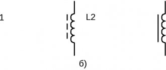
Vector diagram for series connection of elements

To construct vector diagrams, first compose equations according to Kirchhoff's laws for the electrical circuit in question.

Let's consider the electrical circuit shown in Fig. 1, and draw a vector voltage diagram for it. Let us denote the voltage drop across the elements.

Rice. 1. Series connection of circuit elements

Let's create an equation for this chain according to Kirchhoff's second law:

UR + UL + UC = E.

According to Ohm's law, the voltage drop across the elements is determined by the following expressions:

UR = I ∙ R,

UL = I ∙ jXL,

UC = −I ∙ jXC.

To construct a vector diagram, it is necessary to display the terms given in the equation on the complex plane. Typically, current and voltage vectors are displayed on their own scales: separately for voltages and separately for currents.

From the mathematics course we know that j = 1∠90°, −j = 1∠−90°. Hence, when constructing a vector diagram, multiplying a vector by an imaginary unit j results in a rotation of this vector by 90 degrees counterclockwise, and multiplication by −j results in a rotation of this vector by 90 degrees clockwise.

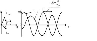
When constructing a vector diagram of voltages on the complex plane, we will first display the current vector I, after which we will display the voltage drop vectors relative to it (Fig. 2), taking into account the above relations for the imaginary unit.

The voltage drop across the resistor UR coincides in direction with the current I (since UR = I ∙ R, and R is a purely real value or, in simple words, there is no multiplication by an imaginary unit). The voltage drop across the inductive reactance leads the current vector by 90° (since UL = I ∙ jXL, and multiplying by j leads to a rotation of this vector by 90° counterclockwise). The voltage drop across the capacitive reactance lags behind the current vector by 90° (since UC = −I ∙ jXC, and multiplying by −j leads to a rotation of this vector by 90° clockwise).

Rice. 2. Vector diagram of voltages for a series connection of circuit elements. Please note that one vector diagram shows only the vectors of those quantities whose frequency coincides!

Vector diagram for parallel connection of elements

Let's consider the electrical circuit shown in Fig. 3, and draw a vector diagram of currents for it. Let us denote the direction of the currents in the branches.

Rice. 3. Parallel connection of circuit elements

Let's create an equation for this chain according to Kirchhoff's first law:

I – IR – IL – IC = 0,

where

I = IR + IL + IC.

Let us determine the currents in the branches according to Ohm’s law using the following expressions, taking into account that 1 / j = −j:

IR = E/R,

IL = E / (jXL) = −j ∙ E / XL,

IC = E / (−jXC) = j ∙ E / XC,

To construct a vector diagram, it is necessary to display the terms given in the equation on the complex plane.

When constructing a vector diagram of currents on the complex plane, we will first display the EMF vector E, after which we will display the current vectors relative to it (Fig. 4), taking into account the above relations for the imaginary unit.

The current in the resistor IR coincides in direction with the emf E (since IR = E / R, and R is a purely real quantity or, in simple words, there is no multiplication by an imaginary unit). The current in the inductive reactance lags behind the EMF vector by 90° (since IL = −j ∙ E / XL, and multiplying by −j results in a rotation of this vector by 90° clockwise). The current in the capacitive reactance leads the EMF vector by 90° (since IC = j ∙ E / XC, and multiplying by j leads to a rotation of this vector by 90° counterclockwise). The resulting current vector is determined after the geometric addition of all vectors according to the parallelogram rule.

Rice. 4. Vector diagram of currents for parallel connection of circuit elements

For an arbitrary circuit, the algorithm for constructing vector diagrams is similar to the above, taking into account the currents flowing in the branches and the applied voltages.

Please note that the site provides a tool for constructing vector diagrams online for three-phase circuits.

1. Resistor

An ideal resistive element has neither inductance nor capacitance. If a sinusoidal voltage is applied to it (see Fig. 1), then the current i

through it will be equal

(1)

Relation (1) shows that the current has the same initial phase as the voltage. Thus, if signals u

and
i,
then the corresponding sinusoids on its screen will pass (see Fig. 2) through zero simultaneously, i.e.
across the resistor, the voltage and current are in phase.
From (1) it follows:

;

Moving from the sinusoidal functions of voltage and current to their corresponding complexes:

;

— divide the first of them by the second:

(2)

The result obtained shows that the ratio of two complexes is a real constant. Consequently, the corresponding voltage and current vectors (see Fig. 3) coincide in direction.

2. Capacitor

An ideal capacitive element has neither active resistance (conductivity) nor inductance. If a sinusoidal voltage is applied to it (see Fig. 4), then the current i

through it will be equal

(3)

The result obtained shows that the voltage across the capacitor lags in phase with the current by
/2.
Thus, if signals
u
and
i
, then on its screen there will be a picture corresponding to Fig. 5.

From (3) it follows:

;

The entered parameter is called the capacitive reactance of the capacitor

.
Like resistive resistance, it has the dimension Ohm
.
However, unlike R
, this parameter is a function of frequency, as illustrated in Fig. 6. From Fig. 6 it follows that at , the capacitor represents a discontinuity for the current, and at .

Moving from the sinusoidal functions of voltage and current to their corresponding complexes:

;

— divide the first of them by the second:

(4)

The last relation is the complex resistance of the capacitor. Multiplying by corresponds to rotating the vector by an angle clockwise. Consequently, equation (4) corresponds to the vector diagram presented in Fig. 7.

3. Inductor

An ideal inductive element has neither active resistance nor capacitance. Let the current flowing through it (see Fig. be determined by the expression. Then for the voltage at the terminals of the inductor we can write

(5)

The result obtained shows that the voltage on the inductor is ahead of the current in phase by
/2
.
Thus, if signals u
and
i
, then on its screen (an ideal inductive element) there will be a picture corresponding to Fig. 9.

From (5) it follows:

The entered parameter is called the inductive reactance of the coil;

its dimension is Om. Like a capacitive element, this parameter is a function of frequency. However, in this case this dependence is linear, as illustrated in Fig. 10. From Fig. 10 it follows that at , the inductor does not provide resistance to the current flowing through it, and at .

Moving from the sinusoidal functions of voltage and current to the corresponding complexes:

;

Let's divide the first of them by the second:

(6)

The resulting relationship is complex

inductor resistance. Multiplying by corresponds to rotating the vector by an angle counterclockwise. Consequently, equation (6) corresponds to the vector diagram presented in Fig. eleven

4. Series connection of resistive and inductive elements

Let in the branches in Fig. 12 . Then

Where

, and the limits of change.

Equation (7) can be associated with the relation

which, in turn, corresponds to the vector diagram in Fig. 13. Vectors in Fig. 13 form a figure called a stress triangle

. Similar expression

can be graphically represented by a resistance triangle

(see Fig. 14), which is similar to a stress triangle.

5. Series connection of resistive and capacitive elements

Omitting intermediate calculations, using relations (2) and (4) for the branch in Fig. 15 can be written down

(8)

Where

, and the limits of change.

Based on equation (7), triangles of voltages (see Fig. 16) and resistances (see Fig. 17), which are similar, can be constructed.

6. Parallel connection of resistive and capacitive elements

For the circuit in Fig. 18 the following relations hold:

;

, where [Sm] – active conductivity;

, where [Sm] is the reactance of the capacitor.

Vector diagram of currents for a given circuit, called a current triangle

, shown in Fig. 19. It corresponds to an equation in complex form

Where ;

— complex conductivity;

Conduction triangle

, similar to the current triangle, is shown in Fig. 20.

For the complex resistance of the circuit in Fig. 18 can be written

It should be noted that the result obtained is similar to the expression known from a physics course for the equivalent resistance of two parallel connected resistors.

7. Parallel connection of resistive and inductive elements

For the circuit in Fig. 21 can be written

;

, where [Sm] – active conductivity;

, where [Sm] is the reactance of the inductor.

The vector diagram of currents (Fig. 22) for a given circuit corresponds to an equation in complex form

Where ;

— complex conductivity;

Conduction triangle

, similar to the current triangle, is shown in Fig. 23.

The expression for the complex resistance of the circuit in Fig. 21 looks like:

Literature

1. Basics

circuit theory: Textbook. for universities / G.V. Zeveke, P.A. Ionkin, A.V. Netushil, S.V. Strakhov. –5th ed., revised. –M.: Energoatomizdat, 1989. -528 p.

2. Bessonov L.A.

Theoretical foundations of electrical engineering: Electric circuits. Textbook for students of electrical engineering, energy and instrument engineering specialties of universities. –7th ed., revised. and additional –M.: Higher. school, 1978. –528 p.

Test questions and tasks

1. What is the essence of reactance?

2. Which element: a resistor, an inductor, or a capacitor can be used as a shunt to observe the shape of the current?

3. Why are inductors and capacitors not used in DC circuits?

4. In the branch in Fig. 12 . Determine the complex resistance of the branch if the current frequency is . Answer: .

5. In the branch in Fig. 15 . Determine the complex resistance of the branch if the current frequency is . Answer: .

6. In the circuit in Fig. 18 . Determine the complex conductivity and resistance of the circuit for .Answer: ; .

7. The current flowing through the inductor changes according to law A.

Determine the complex effective value of the voltage on the coil. Answer: .

Algorithm for creating a ray vector diagram in Excel

To simplify our lesson, let's assume that we are talking about relationships not between fourteen as in the graph, but for now only with 4 people named Anton, Alice, Boris and Bella.

Our matrix of the level of relationships and connections between them looks like this:

0 means no relationship;
1 means weak relationship (for example: Anton and Alice just know each other);
2 means a strong relationship (for example, Boris and Alisa are friends).

How can we geometrically model the visualization of this raw data? If we were to draw the relationship between these four people (Anton, Alice, Boris and Bella), it would schematically look like this:

2 criteria that we need to determine:

Location of dots (where people's names are printed).
Lines (starting and ending points of connecting lines).

Defining and plotting points

First we need to plot our points so that the space between each point is the same. This will create a balanced schedule.

Which geometric figure best satisfies our need for such equal intervals? Of course it's a circle!

You might object that the finished diagram model does not have a circle shape. Yes, really no - that's it. We don't need to draw a circle. We just need to plot the points around it.

So we have 4 stakeholders, we need 4 points:

If we have 12 stakeholders, we need 12 points.
If we have 20, we need 20 points.

Assuming the origin of our circle is (x, y), the radius is r and theta is 360 divided by the number of points we need. The first point (x1, y1) on the circle will be at this position:

x1 = x + r * COS (theta);
y1 = y + r * SIN (theta).

Once all the points are calculated and connected to the XY chart (scatter plot), let's move on.

Drawing lines on a ray diagram

Let's say we have n people in our network. This means that each person can have a maximum of n-1 relationships.

Thus, the total number of possible lines on our graph is n * (n-1) / 2.

We need to divide it by 2, as if A knows B, then B also knows A. But we only need to draw 1 line.

The network graph analysis ray diagram template is configured to work with 20 people. It can be downloaded at the end of the article and used as a ready-made analytical tool for visualizing these connections. This means that the maximum number of rows we can have will be 190.

Each line requires adding a separate series to the chart. This means we need to add 190 series of data for just 20 people. And it only satisfies one line type (dashed or thick). If we want different lines depending on the type of relationship, we need to add another 190 episodes.

It's painful and funny at the same time. Fortunately, there is a way out!

We can use a much smaller number of series and still produce the same graph.

Let's say we have 4 people - A, B, C and D. For the sake of simplicity, let's assume that the coordinates of these 4 people are as follows:

A – (0.0);
B – (0.1);
C – (1,1);
D – (1.0).

And let's say A has relationships with B, C and D.

This means that we need to draw 3 lines, from A to B, from A to C and A to D.

Now, instead of putting 3 series for the chart, what if we put one long series that looks like this:

(0,0), (0,1), (0,0), (1,1), (0,0), (1,0)

This means we simply draw one long line from A to B, A to C, A to D. Granted, it's not a straight line, but Excel scatter plots can draw any line if you give it a set of coordinates.

See this illustration to understand the technique:

So instead of 190 series of data for the chart, we just need 20 series.

In the last chart we have 40 + 2 + 1 series of data. It's because:

20 lines for weak relationships (dashed lines);
20 lines for strong relationships (thick lines);
1 line for highlighting in blue the weak relationships of the selected participant;
1 line for highlighting in green the strong relationships of the selected participant;
1 set without lines, but just dots for data labels on the graph.

How to generate all 20 data series:

This requires the following logic:

Assuming we need lines for person n's relationships.
This person's point will be (Xn, Yn) and has already been calculated earlier (at points on the graph around the circle).
We only need 40 rows of data.
Every odd row will have (Xn, Yn).
For each even row:
divide the line number by 2 to get the person's number (say m>);
(Xn, Yn) if there is no relationship between n and m>;
(Xm, Ym) if there are relations.

We need MOD and INDEX formulas to express this logic in Excel.

Once all line coordinates have been calculated, add them to our scatter plot as new series using the tool from the additional menu: “WORKING WITH DIAGRAMS” - “CONSTRUCTOR” - “Select data” in the “Select data source” window, use the “Add” button to adding all 43 rows.

We will implement the creation of such a ray diagram of connections in 3 stages:

Preparation of initial data.
Data processing.
Visualization.

Preparing data for a ray diagram

As mentioned above, this template will have the ability to visually build connections for up to 20 participants (companies, branches, counterparties, etc.). The template worksheet "Data" provides a table for populating incoming values. For example, let’s fill it out for 14 market participants:

On the same sheet we will create an additional table, which is a matrix of connections of all possible participants, generated by the formula:

With the data preparation completed, we move on to processing.

How to calculate the sum of vectors?

Vectors and matrices in a spreadsheet are stored as arrays.

It is known that the sum of vectors is a vector whose coordinates are equal to the sums of the corresponding coordinates of the original vectors:

To calculate the sum of vectors you need to perform the following sequence of actions:

– Enter the values of the numerical elements of each vector into ranges of cells of the same size.

– Select a range of cells for the calculated result of the same dimension as the original vectors.

– Enter the formula for multiplying ranges into the selected range

– = Vector_Address_1 + Vector_Address_2 Address

– Press the key combination [Ctrl] + [Shift] + [Enter].

Example.

Two vectors are given:

It is required to calculate the sum of these vectors.

Solution:

– To cells in the range A2:A4

Let's enter the values of the coordinates of vector a1, and into the cells of the range
C2:C4
- the coordinates of vector a2.

– Select the cells of the range in which the resulting vector C will be calculated ( E2:E4

) and enter the formula into the selected range:

=A2:A4+C2:C4

– Press the key combination [Ctrl] + [Shift] + [Enter]. In cells in the range E2:E4

the corresponding coordinates of the resulting vector will be calculated.

Vector diagram for a circuit with parallel connections of branches. Vector diagram method

For instantaneous quantities, in accordance with Kirchhoff’s first law, the current equation

Representing the current in each branch as the sum of the active and reactive components, we obtain

For effective currents you need to write a vector equation

The numerical values of the current vectors are determined by the product of the voltage and conductivity of the corresponding branch.

In Fig. 14.14, b a vector diagram corresponding to this equation is constructed. As usual when calculating circuits with parallel connections of branches, the voltage vector U is taken as the initial vector, and then the current vectors in each branch are plotted, and their directions relative to the voltage vector are chosen in accordance with the nature of the conductivity of the branches. The starting point when constructing a current diagram is the point coinciding with the beginning of the voltage vector. From this point the vector l1a of the active current of branch I is drawn (in phase with the voltage), and from its end the vector I1p of the reactive current of the same branch is drawn (leads the voltage by 90°). These two vectors are components of the first branch current vector I1 . Next, the current vectors of other branches are plotted in the same order. It should be noted that the conductivity of branch 3-3 is active , therefore the reactive component of the current in this branch is zero. In branches 4-4 and 5-5, the conductivities are reactive , therefore there are no active components in the composition of these currents.