Determination of active resistance of wires
the active resistance of wires using reference data compiled on the basis of GOST 839-80 - “Bare wires for overhead power lines”, tables 1 - 4. You can find these tables directly in GOST itself, I will give just a few.
It is not recommended to use all known formulas for determining active resistance [L1. p.18], this is due to the fact that the actual cross-section differs from the nominal cross-section, the wires were produced at different times, according to different GOSTs and specifications, and the values of conductivity (ρ) and resistivity (γ) are different:
Where:
- γ – the value of specific conductivity for copper and aluminum wires at a temperature of 20 °C is accepted: for copper wires – 53 m/Ohm*mm2; for aluminum wires – 31.7 m/Ohm*mm2;
- s – nominal wire (cable) cross-section, mm2;
- l – line length, m;
- ρ – the resistivity value is accepted: for copper wires - 0.017-0.018 Ohm*mm2/m; for aluminum wires – 0.026 - 0.028 Ohm*mm2/m, see table 1.14 [L2. p.30].
The active resistance of steel wires cannot be calculated mathematically. Therefore, I recommend using appendices P23 - P25 [L1.] to determine active resistance. p.80,81].
High voltage wires with zero resistance
High-voltage wires with zero R are better and more reliable than conventional ones; due to the use of silicone in them, they do not become hard in the cold, and do not become dry over time and temperature.
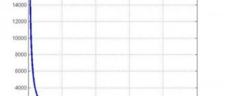
“Zero” high-voltage wires have a difference compared to conventional high-voltage wires with polymer cores: R in them is measured in Ohms and tenths of Ohms, while in ordinary ones it is measured in thousands.
In addition, it has other advantages, primarily a longer service life.
Features of active resistance
Resistance in electrical engineering is the most important parameter by which some part of an electrical circuit resists the current passing through it. The formation of this quantity is facilitated by changes in electricity and its transition to other types of energy states.
This phenomenon is typical only for alternating current, under the influence of which active and reactive resistances of cables are formed. This process represents irreversible changes in energy or its transfer and distribution between individual elements of the chain. If changes in electricity become irreversible, then such resistance will be active, and if metabolic processes take place, it becomes reactive. For example, an electric stove produces heat, which is no longer converted back into electrical energy.
This phenomenon fully affects any type of wire and cable. Under the same conditions, they will resist the passage of direct and alternating current differently. This situation arises due to the uneven distribution of alternating current across the cross-section of the conductor, resulting in the formation of the so-called surface effect.
Linear and wave parameters
20 Single-circuit transposed overhead line with unsplit phase
Lines without phase splitting are being built in our country at They
have only three phase wires, which, in order to ensure equality of reactive parameters, are subjected to a complete cyclic rearrangement over the length of the transposition cycle.
Linear active resistance . The active resistance of wires is their resistance to alternating current, determined taking into account the influence of the surface effect, the presence of longitudinal magnetic flux, losses in the core and twisting of the wires.
assumptions:
— the difference between linear active resistance and ohmic resistance at a frequency of 50 Hz can be neglected;
— the difference between the average operating temperature of the wire and 20°C is not taken into account.
Linear inductive reactance . The magnetic field that occurs around and inside the wire determines its inductive reactance. EMF corresponding to inductive
changing according to a sinusoidal law and having practically no active component, since the losses associated with the reorientation of the dielectric dipoles (in this case, air) are negligible. The values of these currents, called charging currents, are determined by the partial capacitances between the phases and between each phase and the ground. During transposition, the resulting charging current of the phase is determined by the so-called “working” conductivity
Rice. 3. Arbitrary relative arrangement of phases of a single-circuit overhead line
power transmission
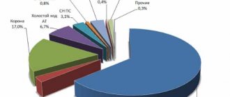
Linear active conductivity . The electrostatic field of the line, under certain conditions, causes ionization of the air layer near the surfaces of the phase wires. This phenomenon, called the corona phenomenon of wires (or the corona phenomenon for short), occurs when the electric field strength on the surface of the wire exceeds a certain critical value. Corona wires are accompanied by acoustic noise and interference with radio and television reception. Active power consumption for air ionization (corona power loss - D P
cor) in the equivalent circuit are taken into account by introducing active conductance of line
(g).
Its linear value
(g0,
S/km) can be approximately determined from the average annual linear values of power losses to the corona (D
P
cor0) and the rated line voltage (
U
n) according to the expression
However, when calculating the modes of 220 kV electrical networks during design, equivalent circuits of lines without active conductivities are usually used, since the resulting error in determining the mode parameters does not exceed the error of the original data. The charging power value is determined by the expression
The characteristic impedance also determines such an important characteristic of a power transmission line as its natural power, which indirectly characterizes the throughput of the line. Therefore, knowledge of this indicator is a kind of guideline for choosing the appropriate rated voltage of sections of a newly designed network.
Natural line power
P
n »
U
n2 /
Z
in .
Cable lines
Structural differences between a cable line and an overhead line (proximity of current-carrying conductors; the presence of solid electrical insulation with a relative dielectric constant significantly greater than that of air; the presence of metal screens and shells surrounding each or all cable conductors, etc.) determine a significant difference in linear parameters of overhead and cable lines at the same nominal voltage and cross-section of current-carrying elements.
Linear active resistance . The assumptions made when determining the linear active resistance of an overhead line are unacceptable in the case of a cable line. Firstly, the influence of the surface effect and the proximity effect, especially in conductors of large cross-sections, is very significant and, accordingly, the active resistance differs significantly from the ohmic one. Secondly, cable lines, as a rule, operate at the maximum permissible or close to them core heating temperatures (up to 85°C) and neglecting their difference from 20°C introduces a noticeable error.
Cable lines 6 - 35 kV are constructed mainly using cables with paper insulation impregnated with a viscous composition, which have both copper and aluminum conductors. For 6 - 10 kV cables, core cross-sections from 10 to 240 mm2 are used. The range of cross-sections of 35 kV cable lines is 120 - 300 mm2 .
Linear reactive parameters . Due to the above-mentioned design features of cable lines, their linear inductive reactance is significantly less, and their linear capacitive conductivity is greater than that of overhead lines. The linear inductive resistance of cable lines 6-220 kV is 2-4 times less than that of overhead lines of the same rated voltages.
The linear capacitive conductivity of cable lines differs from that of overhead lines to an even greater extent. In addition to the convergence of phases in a common shell or shielding of cores, leading to an increase in b0
To the same extent as a decrease in
x
0 (by a factor of 2
- 4), the difference in relative dielectric constant from unity has a significant effect.
Linear active conductivity . In a cable line, active conductivity is determined by active power losses in the cable insulation (dielectric losses) and can be expressed through capacitive conductivity and dielectric loss tangent tgd:
(4.81)
tgd values
determined by the type of insulation of the cable cores.
In practice, dielectric losses in cable lines (due to the smallness of tgd)
have to be taken into account only at voltages of 220 kV and above.
Thus, at Un
= 110 kV, the equivalent circuit of the cable line does not contain branches with active conductivity.
Features of equivalent circuits . In accordance with the above ranges of changes in linear capacitive conductivity, the charging power of 1 km of a 110 kV cable line exceeds the same indicator for an overhead line by 40-50 times in the case of oil-filled cables and by 15-40 times in the case of cables with polyethylene insulation.
At the same time, cable lines, as a rule, have a significantly shorter length compared to overhead lines of the same rated voltage with approximately the same or even slightly higher transmitted powers. Therefore, taking into account in the equivalent circuit of a cable line branches with capacitive conductivity is usually necessary only at lower rated voltages, the cable line is represented with sufficient accuracy by one of the equivalent circuits shown in Fig. 4, which differ in the presence of inductive reactance.
The need to take into account in the equivalent circuit of a cable line its inductive reactance is determined by its relationship with the value of active resistance.
For 110–220 kV cable lines, the question of the possibility of refusing to take into account inductive reactance in the equivalent circuit does not arise.
Wave parameters and natural power . Due to the short length of cable lines, even at voltages of 110–220 kV, their wave properties have no practical significance when calculating their steady-state conditions, therefore their wave parameters are not considered in detail here.
Z value compared to overhead lines of the same rated voltages
in significantly higher. On average, the natural power of cable lines of 110–220 kV is approximately 10 times higher than the corresponding value for the corresponding overhead lines.
22 Transformers
Double winding.
Rice. 3 Equivalent circuit of a two-winding transformer
Three-winding.
Inductive resistance of the transformer windings reduced to basic conditions (in named units):
Active resistance of the transformer windings reduced to basic conditions (in named units):
Rice. 4 Equivalent circuit of a three-winding transformer
Autotransformers.
Short circuit voltage of autotransformer windings:
Inductive resistance of autotransformer windings:
23 Twin reactors
Twin reactor model
Three operating modes of a dual reactor (SR) are possible: through, longitudinal and single-circuit.
I. Let's consider a method for constructing a CP for an end-to-end mode. Passport data used:
Inductive reactance in normal mode ( XL
), Ohm;
Coupling coefficient ( kcv
. = 0.5 by default).
It is proposed to implement the equivalent circuit by a subsystem (see Fig. 1), which includes two inductive reactances, the values of which are determined by the expression:
Fig.1. Double reactor in through operation mode. a) conditional representation of a dual reactor; b) equivalent circuit.
II. SR in longitudinal operating mode.
| Rice. 2. Twin reactor in longitudinal operating mode. a) conditional representation of a dual reactor; b) equivalent circuit. |
| III. CP in single-circuit operating mode. |
| Rice. 3. Double reactor in single-circuit operating mode. a) conditional representation of a dual reactor; b) equivalent circuit. |
Load Characteristics
Asynchronous motors consume active and reactive power from the network. The energy corresponding to the consumed active power is converted by the engine into mechanical energy, which is used to set the machine-tools in motion and perform useful work. The value of the active power taken by the asynchronous motor from the network is determined by the load of the machine-implement.
where P
0,
Q
0,
U
0 – active and reactive power and voltage of the load node in the initial mode;
f
n – nominal frequency value. Index 0 marks the parameters of the initial steady state.
Coefficient values a
,
b
,
c
and
d
in the expressions depend on the degree of “flatness” of the SCN. There are “flat”, “medium” and “steep” characteristics.
The ranges of variation of all these coefficients are quite large, therefore, as an illustration, we present their values for characteristics of average slope, which correspond to the following composition of the node load as a percentage of the total active power:
— large asynchronous motors — 15
— small asynchronous motors — 35
— large synchronous motors — 9
– converters and electric furnaces – 11
— lighting and household load — 22
— losses in networks — 8.
For such a load composition, the average values of the coefficients for active load power are:
In this case, dependence (5.41) takes the form
From (5.41a) it follows that the generalized static characteristics of the active load in the vicinity of the point corresponding to the nominal values of voltage and frequency (U0=Un,f0=fn
), are linear functions of the corresponding operating parameters and are characterized by average regulatory effects
The regulatory effects of the generalized static characteristics of the reactive load in accordance with (5.42) are equal to
bU values
calculated from the average values of the coefficients
aq
and
bq
for loads reduced to busbars of different rated voltages are:
25 Static loads in design diagrams of electrical networks
f = const
.
If it is necessary to take into account changes in load power as a function of voltage, in some cases they use the representation of the load with a constant current ( I
n = const). The active and reactive components of this current are calculated from the given values of load power and voltage in the initial mode.
When calculating modes characterized by significant changes in voltage at network nodes, it is convenient to represent the load in parallel (Fig. 5.19, a) or in series (Fig. 5.19, b) connected by constant active and reactive resistances. The values of these resistances are selected in such a way that the power they determine at normal mode voltage is equal to the specified load power.
Then, with a parallel connection of resistances
(5.44)
and with a serial connection
(5.45)
Where
Rice. 5.20 Generalized dependences of active (1) and reactive (2) load power and
private dependence ( P
*n =
Q
*n) when the load is represented as unchanged and equal in
value of active and inductive resistance (3)
26 Preparation of a design diagram for the electrical power system. Reduction to basic conditions
When solving a number of problems, the calculated equivalent circuit of an electrical power system is an electrical circuit, which, in addition to active and inductive resistances and conductivities, includes ideal transformers (an ideal transformer is characterized by a single parameter - transformation coefficient k
t, in the general case complex), connecting parts of a system of different rated voltages. This scheme is widely used in calculations of steady-state modes, and the results of the calculation are the actual currents of the branches and voltages of the nodes of each stage, which is very convenient for subsequent assessment of the admissibility of the mode, monitoring of certain technical limitations, etc.
To reduce the resistances and conductances of an equivalent circuit to one voltage stage, the following formulas are used:
where k
t
i (i =
1, 2,…,
n) -
transformation ratios of ideal transformers
on the path between the element under consideration and the network of the voltage stage to which reduction is performed (usually this is the stage with the highest voltage), and the assumption is introduced that the transformation ratios of all ideal transformers connecting two voltage stages are real and identical.
In a number of cases, for example in design calculations, when the exact values of transformation ratios are unknown, an approximate reduction using the so-called “average” transformation ratios, equal to the ratio of some average operating voltage values of individual stages (515; 340; 230; 154; 115; 37; 24; 20; 18; 15.75; 13.8; 10.5; 6.3 and 3.15 kV). In this case, recalculation of the resistances and conductances of the voltage step to the kth
steps are made using simpler expressions:
In a number of problems, when, on the one hand, there is no need to know the actual values of the parameters of the modes (for example, when studying stability), and on the other hand, a greater degree of clarity in presenting the results is desirable, it turns out to be advisable to operate not with named, but with dimensionless (relative) units . To convert the parameters of the equivalent circuit and mode into relative units, the basic power values Sb are set,
current
I
b, voltage and resistance
z
b.
Of the four basic quantities, two are independent (can be chosen arbitrarily), the other two are determined from known relationships:
These expressions involve linear values of voltage and current. As a rule, it is convenient to set the values of voltage and power as independent basic quantities and from them determine the basic values of current and resistance. To convert to relative units, the parameter value in named units is divided by the corresponding base value:
27Power quality characteristics
The quality of electricity on power plant buses does not guarantee its quality at the point of consumer connection. It can be different before and after turning on the consumer, and vary depending on the mode of both the power supply system (SES) as a whole and the technological process of the consumer. Electrical receivers and electrical equipment of SES are designed to operate at rated frequency, voltage, current, varying according to a sinusoidal law.
Power quality (QE) standards, i.e. their permissible values in electrical networks of general-purpose power supply systems of alternating three-phase and single-phase current with a frequency of 50 Hz at points to which electrical networks or receivers of electrical energy are connected (points of general connection) are established by the standard - GOST 13109–97.
GOST 13109–97 establishes 11 types of power quality indicators (PQI), which can be divided into three groups.
The first group includes frequency deviations and steady-state voltage deviations. Maintaining these PKEs is possible using system-wide means of frequency and voltage regulation.
The second group includes PCEs that characterize the non-sinusoidal shape of the voltage curve, asymmetry and voltage fluctuations. These are, respectively, the distortion coefficients of the sinusoidal voltage waveform and n
th harmonic component, negative and zero sequence coefficients, voltage fluctuation ranges and flicker dose. The sources of these voltage distortions are electrical receivers.
The third group includes PCEs that characterize random electromagnetic phenomena and electrotechnological processes in the power supply system. These include voltage dips, overvoltages and voltage surges. In most cases, they arise as a result of switching or lightning strikes in a power line.
The CE indicators of the first two groups are standardized by GOST, and two acceptable levels are established for them: normal and limiting.
28 Electrical and technological damage from deterioration of CE
Deterioration of CE leads to a number of negative consequences or damage for certain types of electrical receivers or the consumer as a whole. Damage caused by deterioration of energy efficiency means all types of negative consequences that arise in the operation of solar power plants, consumers and power receivers. Such damage in monetary terms is called economic. There are two types of damage: electrical and technological.
Electrical damage is caused by an increase in electricity losses, a reduction in the service life of electrical equipment and devices, and sudden reversible and irreversible failures of certain technical means.
Technological damage is caused by under-supply and defective products, failures and failures in the operation of electrical equipment, which lead to disruption of production technology.
The listed types of damage should be considered unacceptable. Let's consider the causes and consequences of deterioration of CE, which lead to damage, depending on the type of CE.
29 Frequency deviation
The normally permissible and maximum permissible frequency deviation D / is ±0.2 and ±0.4 Hz, respectively. The reason for the frequency deviation is a change in the active power balance. Rotating machines are most sensitive to frequency deviations. The share of asynchronous motors (IM) from the total load of SPP is approximately 60%. A decrease in frequency leads to a decrease in the rotation speed of the motor, which drives production mechanisms, which contributes to technological damage.
Engine power PºМ
=a
/" is proportional to the moment on its shaft, determined by the characteristics of the driven mechanism. For machine tools, piston pumps n = 1, and for centrifugal pumps and fans n = 2¸4.
As the frequency decreases, the resistance of the IM decreases and the current it consumes increases, which leads to additional heating of the stator and rotor and, as a consequence, to electrical damage caused by a reduction in the service life of the IM due to accelerated wear of its insulation at elevated temperatures.
As the frequency decreases, the reactive power consumption also increases. In Fig. Table 5.1 shows the generalized static characteristics of an asynchronous load. An increase in reactive power consumption contributes to an increase in electricity losses in power lines and transformers, which also leads to electrical damage.
Rice. 5.1 Static characteristics of an asynchronous motor by frequency
30 Voltage deviation
However, GOST 13109-97 establishes the normal and maximum permissible steady-state voltage deviation dU
= ±5% and limit ±10% of the rated network voltage.
Positive voltage deviations lead to a decrease in voltage losses and an increase in power losses in networks, increasing the productivity of mechanisms with asynchronous drives. However, the service life of the equipment is reduced. This especially applies to incandescent lamps. Negative voltage deviations mainly affect performance degradation, increased voltage loss and reduced power loss.
The regulating effect of the load is the change in the consumed active and reactive power of the load as a percentage when the voltage changes by 1%.
Rice. 5.2 Generalized static characteristics of complex stress load
When the voltage across the load decreases, as follows from the static characteristics, the regulating effect of the load helps maintain the voltage at the receiving end of the line, i.e. on the load, due to a reduction in power consumption and, consequently, voltage losses in the line. This is the positive regulatory effect of the load.
As the voltage decreases, the amplitude of the characteristic decreases,
its sliding s
and the rotation speed decreases.
When the IM is stopped, for example, during a deep voltage dip, the possibility of self-start is eliminated, which may be very necessary for some technological processes. An asynchronous motor does not start in cases where a decrease in the stability safety factor of an asynchronous motor can lead to its stalling when k
<1.
As slip increases, the current increases, which leads to additional heating of the IM. During continuous operation at U
= 0.9
U
nom. The service life of the motor is reduced by half (electrical damage).
An increase in voltage leads to an increase in reactive power consumption and corresponding losses in the distribution network. On average, with an increase in voltage by 1%, the consumed reactive power (regulatory effect) increases by 3% for IM with a power of 20–100 kW and by 5–7% for IM of lower power.
31 Voltage fluctuations
Voltage fluctuations in networks occur mainly during the operation of sharply variable loads: controlled thyristor converters with a wide range and high speed of voltage regulation, chipboards, powerful welding units, etc.
Voltage fluctuations negatively affect the visual perception of objects, graphic images and, ultimately, the productivity and vision of workers. With voltage change ranges of more than 10%, gas-discharge lamps may go out; with large ranges (over 15%), the contacts of magnetic starters may fall off. With such fluctuations, failure of capacitors and valves of converter units is observed.
Voltage fluctuations negatively affect the operation of consumers. Thus, at one of the enterprises, to which 10 kV busbars were connected chipboard-40, induction furnaces and high-frequency converting units, the range of voltage changes reached 12%. At the same time, defects in the products of high-frequency heating installations arose and the cores of induction melting furnaces were destroyed, automatic control systems and synchronous electric motors were turned off.
When voltage fluctuations occur, the productivity of electrolysis plants decreases and their service life is reduced due to increased wear of the anodes. At chemical fiber factories, due to fluctuations in the rotation speed of asynchronous motors of winding devices, synthetic threads break or become of different thicknesses, which leads to defects or under-supply of products.
32 Non-sinusoidal voltage
Non-sinusoidal voltage affects all types of electrical receivers.
In particular, zero-sequence currents create additional magnetization of steel in electrical machines, which leads to deterioration of the characteristics of these electric drives and additional heating of the IM stators and magnetic cores of transformers. Typically, higher voltage harmonics, summed with the fundamental harmonic, contribute to an increase in the effective voltage value at the ED terminals.
Higher harmonics of voltage and current adversely affect electrical equipment, creating additional losses in electrical machines, transformers and networks, worsening the operating conditions of capacitor banks (CB), reducing the service life of the insulation of electrical machines and devices, increasing the accident rate in cable networks, causing system failures relay protection, automation, telemechanics and communications.
Higher harmonics of voltage and current also affect the values of power factor and torque of electric motors. In networks of enterprises, large industrial centers, as well as networks of electrified railway transport, these losses can reach 10–15% of the main technical losses.
Capacitor banks and cables are especially sensitive to the appearance of higher harmonics. In capacitors, losses are proportional to the frequency of the applied voltage D P
(
n
) =
U
(2
n
)
n
w
Ctg
d, which leads to their additional heating.
Limitations on additional heating of the CB are set by a permissible increase in the voltage acting at its terminals to 10% U
nom.
and effective current value up to 30% I
nom. .
Cables whose dielectric quality is characterized by leakage current, which determines losses in cable insulation, are similarly susceptible to higher harmonics. Measurements have shown that at kU
= 6.85% over 2.5 years, the leakage current increases by 36%, and
after 3.5 years by 43%.
With a non-sinusoidal voltage, accelerated aging of the insulation of electrical machines, transformers, capacitors and cables is observed as a result of increased heating of current-carrying parts, as well as irreversible physical and chemical processes occurring under the influence of electric fields created by higher current harmonics.
Voltage unbalance
The main sources of negative sequence voltage asymmetry in three-phase solar power plants are: EAFs, induction furnaces, electroslag remelting furnaces, AC traction substations (27 kV), converters with asymmetrical control, and welding installations. Some typical values of negative sequence voltage unbalance coefficients ( k
2
U
) created by such EPs are given in Table. 5.1.
Normal and maximum permissible values of the negative sequence voltage asymmetry coefficient to 2 and
according to GOST 13109-97 for networks of all rated voltages are ±2 and ±4%, respectively.
As can be seen from the table, for many electrical receivers to 2
and either close to these values or significantly exceed them.
Unbalance of the three-phase voltage system leads to the occurrence of negative sequence currents I
2
U
- wire networks - zero-sequence currents
I
0
U.
Currents I
2
U
cause additional heating of rotating machines, creating
negative torque reduces the rotation speed of the rotors of asynchronous motors and the performance of the mechanisms they drive. Reducing the rotation speed, i.e. An increase in IM slip is accompanied by an increased consumption of reactive power and, as a consequence, a decrease in voltage.
With a voltage asymmetry of 2%, the service life of asynchronous motors due to additional losses of active power is reduced by 10.8%, synchronous motors by 16.2%, transformers by 4%, capacitors by 20%. In order to avoid additional heating, the motor load (shaft torque) must be reduced.
According to IEC 892, the rated motor load is allowed at k
2
U
<1% .
At a negative sequence ratio of 2% the motor load should be reduced to 96%, at 3% to 90%, at 4% to 83% and at 5% to 76%. These figures are valid provided that the engine operates with a constant load, i.e. in steady thermal conditions.
34 Voltage sags
To ensure the reliability of power supply, according to the PUE classification, three categories have been established.
Electric receivers of the first category include those whose power supply interruption may entail a danger to human life, a threat to state security, significant material damage, disruption of a complex technological process, disruption of the functioning of particularly important elements of public utilities, communications and television facilities.
Electric consumers of the second category include those whose power supply interruption leads to a massive undersupply of products, massive downtime of workers, machinery and industrial vehicles, and disruption of the normal activities of a significant number of urban and rural residents.
Electrical receivers of the third category are all others that do not fall within the definition of the first and second categories. In such industries as electric power, petrochemical, metallurgical and mechanical engineering, a break in the technological cycle is unacceptable.
What is resistance, its nature
Resistance (denoted by the Latin letter R) is one of the main characteristics of conductors. Depending on the application, this property can play both a positive and negative role when using a conductor.
First of all, metals and metal alloys can be conductors. Atoms in a metal have free electrons, which are charge carriers. Electrons in a metal are constantly moving randomly from atom to atom. If an electric current is connected to them, their movement becomes orderly. When an electron collides with an atomic structure, the electron transfers its energy to the metal, thereby heating it. The more structural obstacles in the path of the electron, the greater the R of the metal.
Lossless line
Fig.6. Diagrams of voltage, current and input resistance in a short-circuited line
In a lossless line, the linear parameters R
1 = 0 and
G
1 = 0. Therefore, for the propagation coefficient
γ
and wave resistance
W
we obtain:
| ; . | (20) |
Taking this into account, expressions for voltage and current (15) will take the form:
| (21) |
When deriving these relations, the features[11] of hyperbolic functions[8] were taken into account.
Let's look at specific examples of line operation without losses for the simplest loads.
Open line
In this case, the current flowing through the load is zero ( I
H = 0), therefore the expressions for voltage, current and input resistance in the line take the form:
| (22) |
Fig.7. Diagrams of voltage, current and input resistance in a short-circuited line
In Fig. 6 these dependencies are illustrated graphically. From relations (22) and graphs it follows:
- in a line open at the end, a standing wave mode is established, voltage, current and input resistance along the line change according to a periodic law with a period of λ
L/2;
the input resistance of the open line is purely imaginary except for points with coordinates z
=
nλ
L/4,
n
= 0,1,2,…;
if the length of an open line is less than λ
L/4, then such a line is equivalent to a capacitance;
an open line at the end with a length of λ
L/4 is equivalent to a series resonant circuit at the frequency under consideration and has zero input resistance;
a line whose length lies in the range from λ
L/4 to
λ
L/2 is equivalent to inductance;
an open line at the end with a length of λ
L/2 is equivalent to a series resonant circuit at the frequency in question and has an infinitely large input resistance.
Closed line
In this case, the voltage across the load is zero ( U
H = 0), so the voltage, current and input resistance in the line take the form:
| (23) |
In Fig. 7 these dependencies are illustrated graphically.
Fig.8. Diagrams of voltage, current and input resistance in a line loaded with a capacitor
Using the results of the previous section, it is not difficult to independently draw conclusions about the transforming properties of a short-circuited line. Let us only note that a standing wave regime is also established in a closed line. A segment of a short-circuited line with a length less than λ
L/4 has an inductive nature of the input resistance, and with a length
λ
L/4 such a line has an infinitely large input resistance at the operating frequency [12].
Capacitive load
As follows from the analysis of open line operation, each capacitance C
at a given frequency
ω,
λ
can be assigned .
Capacitance C
has capacitance.
Let us equate the value of this resistance to the input resistance of an open line of length l
< λ
L/4:
.
From here we find the line length equivalent to the input resistance of the capacitance C
:
.
Knowing the diagrams of voltage, current and input resistance of an open line, we restore them for a line operating on capacitance (Fig. 8). From the diagrams it follows that a standing wave mode is established in the line operating on the capacitance.
When the capacitance changes, the diagrams shift along the z
. In particular, as the capacitance increases, the capacitance decreases, the voltage across the capacitance drops, and all diagrams shift to the right, approaching the diagrams corresponding to the short-circuited line. As the capacity decreases, the diagrams shift to the left, approaching the diagrams corresponding to the open line.
Inductive load
Fig.9. Diagrams of voltage, current and input resistance in a line operating inductance
As follows from the analysis of the operation of a closed line, each inductance L
at a given frequency
ω,
λ
can be assigned .
Inductance L
has inductive reactance
iX
L =
iωL
.
Let us equate this resistance to the input resistance of a closed line of length λ
L/4:
.
From here we find the line length l
, equivalent in input resistance to inductance
L
:
.
Knowing the diagrams of voltage, current and input resistance of a line closed at the end, we restore them for a line operating in inductance (Fig. 9). It follows from the diagrams that a standing wave mode is also established in the line operating with inductance. A change in inductance leads to a shift in diagrams along the z
.
Moreover, with an increase in L,
the diagrams shift to the right, approaching the idle speed diagrams, and with a decrease
in L
, to the left along the
z
, tending to the short circuit diagrams.
Active load
In this case, the current and voltage across the load R
H are related by the relation
U
H =
I
H
R
H [13]. Expressions for voltage and current in line (21) take the form:
| (23) |
Let's consider the operation of such a line using voltage analysis as an example. Let us find from (23) the voltage amplitude in the line:
| (24) |
It follows that three cases can be distinguished:
- The load resistance is equal to the characteristic impedance of the line R
Н =
W
[9][10] The load resistance is greater than the characteristic impedance of the line
R
Н >
W
The load resistance is less than the characteristic impedance of the line
R
Н < W
In the first case, from (24) it follows | U
|
= U
N, that is, the distribution of the voltage amplitude along the line remains constant, equal to the voltage amplitude at the load. This corresponds to the traveling wave mode in the line.
Inductive reactance
The alternating magnetic field created during energy transfer becomes a source of reactance of this type.
The inductive option mainly depends on the characteristics of the current passing, the diameter and distance between the wires. The resistance itself is usually classified as follows:
- depending on current parameters and material - internal;
- due to the geometric features of the line - external. In this case, this indicator will be a constant value, independent of any other factors.
Cable factories always indicate information about inductive reactance in their catalogs.
This parameter is usually determined by the following expression:
in which the inductive indicator for 1 km of wire is , and L is the length.
X kilometer section is calculated using the following formula:
Where: Dav – average distance along the central axis of the existing wires, mm; d – diameter of the working conductor, mm; μt – relative magnetic permeability.
Long line input impedance
Input impedance
line - is an important characteristic, which is determined in each section of the line as the ratio of voltage to current in this section:
| (19) |
Since the voltage and current in the line change from section to section, the input resistance of the line also changes relative to its longitudinal coordinate z
. In this case, they talk about the transforming properties of the line, and the line itself is considered as a resistance transformer. The property of a line to transform resistance will be discussed in more detail below.
ACTIVITY
- Video surveillance
Order an estimate - Security alarm
Order a quote - Access control
Order a quote - Fire alarm
Order a quote - Fire extinguishing
Order an estimate - Fireproof barriers
Order a quote - Fire retardant treatment
Request a quote - Category calculation
Order calculation - Automation
Order calculation - Frequency drive
Order calculation - Energy metering
Order a calculation - Lightning protection, Grounding
Order calculation - Electrical installation
Order an estimate - Local networks and SCS
Order a calculation - Satellite communications
Order a quote - Audio and video systems
Order a quote
Calculation of inductive and capacitive reactance is carried out using the formulas:
XC=1/(2π×F×C); XL=2π×F×L
X L - Inductive reactance, (Ohm)
X C - Capacitance, (Ohm)
F — Signal frequency, (Hz)
The calculation will be valid only for a sinusoidal current.
To calculate any parameter, you must enter two other values.
| Calculation of inductive and capacitive reactance | |
| Units of measurement when calculating capacity: | kHz, nF, Ohm MHz, pF, Ohm |
| Units of measurement when calculating inductance: | kHz, mH, Ohm MHz, μH, Ohm |
| Signal frequency: | |
| Value (capacitance or inductance): | |
| Reactance: | |
| *Input format – x.xx (delimiter – dot) |
| Please send your wishes, comments, recommendations for improving the calculations section on our website by email [email protected] Copying java scripts is permitted provided a link to the source is provided. |
ALL CALCULATIONS
Physical and technical data of conductor material
| Material | Specific active resistance ρ, Ohm∙mm2/km | Melting temperature t, оС | Density δ, g/cm3 |
| Steel | 7,9 | ||
| Al | 29,5—31,5 | 2,7 | |
| Si | 18,5—19,0 | 8,7 | |
| Ai | 19,3 | ||
| Ag | 10,5 | ||
| Pt | 20,5 |
Table P 1.2
Electrical parameters of AMKA insulated wires
| Wire brand | Conductors | Zero core | Current of the established mode at t = 25°C, A | ||
| DC resistance +20°С, Ohm/km | Positive sequence reactance. Ohm/km | Zero sequence reactance, Ohm/km | Direct current resistance +20°C, Ohm/km | Zero sequence reactance, Ohm/km | |
| 1×16+25 | 1,91 | 0,090 | — | 1,38 | 0,074 |
| 3×16+25 | 1,91 | 0,108 | 0,055 | 1,62 | 0,074 |
| 4×16+25 | 1,21 | 0,108 | 0,030 | 0,380 | 0,074 |
| 3×25+35 | 1,20 | 0,106 | 0,045 | 0,986 | 0,073 |
| 4×25+35 | 1,20 | 0,106 | 0,025 | 0,966 | 0,074 |
| 3×35+50 | 0,868 | 0,104 | 0,045 | 0,720 | 0,073 |
| 3×50+70 | 0,641 | 0,101 | 0,045 | 0,493 | 0,071 |
| 3×70+95 | 0,433 | 0,097 | 0,045 | 0,363 | 0,070 |
| 3×120+95 | 0,253 | 0,092 | 0,030 | 0,363 | 0,078 |
Note. Symbols of the “AMKA” wire, consisting of 3 cores of phase wires with a cross-section of 16 mm2 and one carrier neutral wire with a cross-section of 25 mm2: 3×16+25
Table P 1.3
Design characteristics of cables with plastic insulation
| Cable brand | Nominal cross-section of cores, mm2 | Specific inductive reactance Ho, Ohm/km | Specific capacitive power q0, kvar/km | |||||||||
| Rated voltage, kV | ||||||||||||
| 0,66 | 0,66 | 0,66 | ||||||||||
| APVG | 2,5—50 | 1,5—240 | — | — | 0,052 | 0,058 | — | — | 1,7 | — | — | — |
| AVVG | 2,5—50 | 1,5—240 | — | — | 0,052 | 0,058 | — | — | 1,7 | 2,1 | — | — |
| VVG | 1,5—50 | 1,5—240 | — | — | 0,041 | 0,048 | — | — | 2,0 | 2,5 | — | — |
| AVVGz | 2,5—50 | 2,5—0 | — | — | 0,052 | 0,058 | — | — | 1,8 | 1,8 | — | — |
| VVGz | 1,5—50 | 1,5—50 | — | — | 0,039 | 0,045 | 2,0 | 2,1 | — | — | ||
| AVBbShv | 4—50 | 6—240 | 6—240 | — | 0,043 | 0,047 | 0,051 | — | 2,0 | 2,2 | 2,5 | — |
| VBBShv | — | — | — | 35— 240 | — | — | — | 0,052 | — | — | — | 2,4 |
Table P 1.4
Design characteristics of three-core paper-insulated cables
| Nominal cross-section mm2 | Active resistance of cores at +20C | Specific inductive reactance X, Ohm/km | Specific capacitive power qo, kvar/km | |||||||
| Rated cable voltage, kV | ||||||||||
| Aluminum | Copper | UP TO 1 | ||||||||
| 3,10 | 1,84 | 0,0730 | 0,110 | 0,122 | — | — | 2,3 | — | — | — |
| 1,94 | 1,15 | 0,0675 | 0,102 | 0,113 | — | — | 2,6 | 5,9 | — | — |
| 1,24 | 0,74 | 0,0662 | 0,091 | 0,099 | 0,135 | — | 4,1 | 8,6 | 24,8 | — |
| 0,89 | 0,52 | 0,0637 | 0,087 | 0,095 | 0,129 | — | 4,6 | 10,7 | 27,6 | — |
| 0,62 | 0,37 | 0,0625 | 0,083 | 0,090 | 0,119 | — | 5,2 | 11,7 | 31,8 | — |
| 0,443 | 0,26 | 0,0612 | 0,080 | 0,086 | 0,116 | 0,137 | 6,6 | 13,5 | 35,9 | 86,0 |
| 0,326 | 0,194 | 0,0602 | 0,078 | 0,083 | 0,110 | 0,126 | 8,7 | 15,6 | 40,0 | 95,0 |
| 0,258 | 0,153 | 0,0602 | 0,076 | 0,081 | 0,107 | 0,120 | 9,5 | 16,9 | 42,8 | 99,0 |
| 0,206 | 0,122 | 0,0596 | 0,074 | 0,079 | 0,104 | 0,116 | 10,4 | 18,3 | 47,0 | |
| 0,167 | 0,099 | 0,0596 | 0,073 | 0,077 | 0,101 | 0,113 | 11,7 | 20,0 | 51,0 | |
| 0,129 | 0,077 | 0,0587 | 0,071 | 0,075 | — | — | 13,0 | 21,5 | 52,8 | |
| 0,105 | 0,062 | — | 0,063 | 0,066 | — | — | — | — | 57,6 | |
| 0,078 | 0,047 | — | — | — | 0,092 | — | — | — | 64,0 | — |
Table P 1.5
Permissible continuous power (heating) of cable lines 6 - 10 kV, MB ∙ A
| Core cross-section, mm2 | Paper insulated cables | Plastic insulated cables | |||||
| 6kV | 10 kV | 6kV | |||||
| In the ground | In the air | In water | In the ground | In the air | In water | In the ground | In the air |
| Copper conductors | |||||||
| 0,7 | 0,6 | 0,9 | — | — | — | 0,9 | 0,6 |
| 0,9 | 0,8 | 1,3 | 1,6 | 1,3 | 2,0 | 1,1 | 0,7 |
| 1,3 | 1D | 1,7 | 1,9 | 1.8 | 2,5 | 1,4 | 0,9 |
| 1,5 | 1,5 | 2,0 | 2,4 | 2,2 | 3,1 | 1,8 | 1,1 |
| 2,0 | 1,8 | 2,5 | 2,9 | 2,7 | 3,9 | 2,1 | 1,6 |
| 2,4 | 2,3 | 3,1 | 3,5 | 3,5 | 4,5 | 2,7 | 1,8 |
| 2,8 | 2,7 | 3,7 | 4,3 | 4,2 | 5,7 | 3,2 | 2,3 |
| 3,4 | 3,2 | 4,3 | 5,0 | 4,8 | 6,6 | 3,7 | 2,7 |
| 3,8 | 3,7 | 5,0 | 5,8 | 5,5 | 7,5 | 4,2 | 3,1 |
| 4,3 | 4,2 | 5,6 | 6,5 | 6,3 | 8,5 | 4,8 | 3,6 |
| 4,9 | 4,8 | 6,4 | 7,5 | 8,2 | 9,8 | 5,6 | 4,0 |
| Aluminum conductors | |||||||
| 0,6 | 0,5 | 0,7 | — | — | 0,7 | 0,4 | |
| 0,7 | 0,6 | 0,9 | 1,0 | 0,9 | 1,6 | 0,9 | 0,6 |
| 0,9 | 0,9 | 1,3 | 1,5 | 1,3 | 1,9 | 1,1 | 0,8 |
| 1,3 | 1,0 | 1,5 | 1,9 | 1,8 | 2,4 | 1,3 | 0,9 |
| 1,5 | 1,4 | 2,0 | 2,3 | 2,0 | 2,9 | 1,7 | 1,1 |
| 1,8 | 1,7 | 2,4 | 2,7 | 2,5 | 3,5 | 2,0 | 1,4 |
| 2,2 | 2,1 | 2,8 | 3,4 | 3,1 | 4,3 | 2,5 | 1,8 |
| 2,5 | 2,4 | 3,4 | 3,9 | 3,6 | 5,0 | 2,8 | 2,0 |
| 2,9 | 2,7 | 3,8 | 4,5 | 4,1 | 5,7 | 3,3 | 2,5 |
| 3,4 | 3,1 | 4,3 | 5,0 | 4,6 | 6,6 | 3,7 | 2,7 |
| 3,8 | 3,7 | 4,9 | 5,8 | 5,5 | 7,6 | 4,2 | 3,1 |
Table P 1.6
Permissible continuous power (heating) of cable lines 20 - 35 kV, MB ∙ A
| Core cross-section, mm2 | 20 kV | 35 kV | |||
| In the ground | In the air | In water | In the ground | In the air | In water |
| Copper conductors | |||||
| 3,6 | 2,7 | 3,9 | — | — | — |
| 4,4 | 3,3 | 4,7 | — | — | — |
| 5,4 | 3,9 | 5,9 | — | — | — |
| 6,6 | 4,9 | 7,4 | — | — | — |
| 7,9 | 5,9 | 9,0 | — | — | — |
| 9,1 | 6,7 | 10,1 | 16,4 | 17,2 | 18,1 |
| 10,1 | 7,6 | 11,0 | 18,6 | 19,5 | 20,6 |
| 11,6 | 8,6 | 12,7 | — | — | — |
| Aluminum conductors | |||||
| 2,7 | 2,1 | 2,9 | — | — | — |
| 3,5 | 2,4 | 3,9 | — | — | — |
| 4,1 | 3,0 | 4,5 | — | — | — |
| 5,0 | 3,8 | 5,7 | — | — | — |
| 6,1 | 4,5 | 6,8 | — | — | — |
| 6,8 | 5,3 | 8,0 | 13,0 | 13,5 | 14,3 |
| 7,9 | 5,7 | 8,9 | 14,3 | 15,1 | 15,8 |
| 9,0 | 6,7 | 9,8 | — | — | — |
Table P 1.7
Active and internal inductive reactances
Single-wire steel wires, Ohm/km
| Current, A | PSO 3.5 | PSO 4 | PSO 5 | |||
| R0 | X”0 | R0 | X”0 | R0 | X”0 | |
| 0,5 1,5 | 14,90 15,20 15,70 16,10 17,40 18,50 20,10 21,40 21,50 21,70 21,80 21,90 20,20 — | 1,04 2,27 4,24 6,45 9,60 11,90 14,10 16,30 16,50 16,70 16,90 17,10 18,30 — | 11,50 11,80 12,30 12,5 13,40 14,3 15,50 16,50 17,30 18,0 18,10 18,10 17,30 — | 0,69 1,54 2,82 4,38 7,90 9;70 11,50 12,50 13,20 14,20 14,30 14,30 13,30 — | — — 7,90 8,35 9,80 10,80 12,30 13,80 15,0 15,40 15,20 14,60 13,60 12,70 | — — 2,13 3,58 6,45 8,10 9,70 11,20 12,30 13,30 13,10 12,40 11,40 10,50 |
Table P 1.8
Active and internal inductive reactances
Steel stranded wires, Ohm/km
| Current, A | Active and internal inductive resistance of the wire, Ohm/km | ||||||||
| PS 25 PMS25 | PS 35 PMS35 | PS 50 PMS50 | PS 70 PMS70 | PS 95 PMS95 | |||||
| R0 | X”0 | R0 | X”0 | R0 | X”0 | R0 | X”0 | R0 | X”0 |
| 5,25 | 0,54 | 3,66 | 0,33 | 2,75 | 0,23 | 1,70 | 0,16 | 1,55 | 0,08 |
| 5,27 | 0,55 | 3,66 | 0,35 | 2,75 | 0,24 | 1,70 | 0,17 | 1,55 | 0,08 |
| 5,28 | 0,56 | 3,67 | 0,36 | 2,75 | 0,25 | 1,70 | 0,17 | 1,55 | 0,08 |
| 5,30 | 0,59 | 3,69 | 0,37 | 2,75 | 0,25 | 1,70 | 0,18 | 1,55 | 0,08 |
| 5,32 | 0,63 | 3,70 | 0,40 | 2,75 | 0,26 | 1,70 | 0,18 | 1,55 | 0,08 |
| 5,35 | 0,67 | 3,71 | 0,42 | 2,75 | 0,27 | 1,70 | 0,19 | 1,55 | 0,08 |
| 5,37 | 0,70 | 3,73 | 0,45 | 2,75 | 0,27 | 1,70 | 0,19 | 1,55 | 0,08 |
| 5,40 | 0,77 | 3,75 | 0,48 | 2,76 | 0,28 | 1,70 | 0,20 | 1,55 | 0,08 |
| 5,45 | 0,84 | 3,77 | 0,51 | 2,77 | 0,20 | 1,70 | 0,20 | 1,55 | 0,08 |
| 5,50 | 0,93 | 3,80 | 0,55 | 2,78 | 0,30 | 1,70 | 0,21 | 1,55 | 0,08 |
| 5,97 | 1,33 | 4,02 | 0,75 | 2,80 | 0,35 | 1,70 | 0,23 | 1,55 | 0,08 |
| 6,70 | 1,63 | 4,80 | 1,16 | 2,85 | 0,42 | 1,72 | 0,25 | 1,55 | 0,09 |
| 6,97 | 1,91 | 5,20 | 1,45 | 2,95 | 0,49 | 1,74 | 0,27 | 1,55 | 0,09 |
| 7,10 | 2,01 | 5,50 | 1,66 | 3,10 | 0,59 | 1,77 | 0,30 | 1,56 | 0,09 |
| 7,10 | 2,06 | 5,60 | 1,73 | 3,25 | 0,69 | 1,79 | 0,33 | 1,56 | 0,09 |
| 7,02 | 2,09 | 5,65 | 1,78 | 3,4 | 0,80 | 1,83 | 0,37 | 1,57 | 0,10 |
| 6,92 | 2,08 | 5,63 | 1,80 | 3,52 | 0,91 | 1,88 | 0,41 | 1,57 | 0,11 |
| 6,85 | 2,07 | 5,60 | 1,80 | 3,61 | 1,00 | 1,93 | 0,45 | 1,57 | 0,11 |
| 6,70 | 2,00 | 5,45 | 1,77 | 3,69 | 1,10 | 2,07 | 0,55 | 1,58 | 0,13 |
| 6,60 | 1,90 | 5,00 | 1,64 | 3,73 | 1,14 | 2,21 | 0,65 | 1,61 | 0,15 |
| 6,5 | 1,79 | 4,89 | 1,57 | 3,70 | 1,15 | 2,27 | 0,70 | 1,61 | 0,17 |
| 6,40 | 1,73 | 5,15 | 1,55 | 3,68 | 1,14 | 2,29 | 0,72 | 1,67 | 0,20 |
| 6,32 | 1,67 | 5,05 | 1,48 | 3,56 | 1,13 | 2,33 | 0,73 | 1,71 | 0,23 |
| 6,07 | 1,52 | 4,85 | 1,35 | 3,58 | 1,04 | 2,33 | 0,73 | 1,83 | 0,31 |
| 5,88 | 1,51 | 4,70 | 1,34 | 3,50 | 0,95 | 2,38 | 0,73 | 1,87 | 0,34 |
| — | — | — | — | 3,45 | 0,94 | 2,23 | 0,71 | 1,89 | 0,35 |
| 5,20 | 1,04 | 4,15 | 0,92 | 3,25 | 0,75 | 2,19 | 0,69 | 1,88 | 0,35 |
| 4,75 | 0,57 | 3,80 | 0,50 | 2,95 | 0,50 | 2,05 | 0,58 | 1,75 | 0,29 |
| 4,62 | 0,30 | 3,70 | 0,27 | 2,8 | 0,31 | 1,90 | 0,45 | 1,65 | 0,27 |
| 4,62 | 0,24 | 3,70 | 0,21 | 2,65 | 0,21. | 1,75 | 0,21 | 1,50 | 0,21 |
Table P 1.9
Linear active resistance of aluminum and steel-aluminum wires
| Wire brand | Weight 1 km of wire, kg | Outer diameter of wire, mm | Continuously permissible load current, A | Linear active resistance Ro, Ohm/km |
| Outdoors | Indoors | |||
| Aluminum wires | ||||
| A 16 | 5,1 | 1,98 | ||
| A 25 | 6,4 | 1,28 | ||
| A 35 | 7,5 | 0,92 | ||
| A 50 | 9,0 | 0,64 | ||
| A 70 | 10,7 | 0,46 | ||
| A 95 | 12,4 | 0,34 | ||
| A 120 | 14,0 | 0,27 | ||
| A 150 | 15,8 | 0,21 | ||
| A 185 | 17,5 | 0,17 | ||
| Steel-aluminum wires | ||||
| AC 10 | 4,4 | 3,120 | ||
| AC 16 | 5,4 | 2,060 | ||
| AC 25 | 6,6 | 1,38 | ||
| AC 35 | 8,4 | 0,850 | ||
| AC 50 | 9,6 | 0,650 | ||
| AC 70 | 11,4 | 0,460 | ||
| AC 95 | 13,5 | 0,33 | ||
| AC 120 | 15,2 | 0,270 | ||
| AC 150 | 17,0 | 0,210 | ||
| AC 185 | 19,0 | 0,170 | ||
| AC 240 | 21,6 | 0,130 | ||
| AC 300 | 23,5 | 0,108 | ||
| AC 400 | 27,2 | 0,080 | ||
| AC 500 | 30,2 | 0,065 | ||
| AC 600 | 33,1 | 0,055 | ||
| ACO 700 | 37,1 | 0,044 | ||
| ASU 120 | 15,5 | — | 0,288 | |
| ASU 150 | 17,6 | — | 0,210 | |
| ASU 185 | 19,6 | — | 0,170 | |
| ASU 240 | 22,4 | — | 0,131 | |
| ASU 300 ASU 400 | 25,2 29,0 | — — | 0,106 0,079 |
Table P 1.10
Inductive reactance of overhead lines with aluminum wires
| Dav, m | Specific inductive resistance Ho, Ohm/km for wires | |||||||||
| A 16 | A 25 | A 35 | A 50 | A 70 | A 95 | A 120 | A 150 | A 185 | A 240 | |
| 0,4 | 0,333 | 0,319 | 0,308 | 0,297 | 0,283 | 0,274 | — | — | — | — |
| 0,6 | 0,358 | 0,345 | 0,336 | 0,325 | 0,309 | 0,300 | 0,292 | 0,287 | 0,280 | — |
| 0,8 | 0,377 | 0,363 | 0,352 | 0,341 | 0,327 | 0,318 | 0,310 | 0,305 | 0,298 | — |
| 1,0 | 0,391 | 0,377 | 0,366 | 0,355 | 0,341 | 0,332 | 0,324 | 0,319 | 0,313 | 0,305 |
| 1,5 | 0,416 | 0,402 | 0,391 | 0,380 | 0,366 | 0,357 | 0,349 | 0,344 | 0,338 | 0,330 |
| 2,0 | 0,435 | 0,421 | 0,410 | 0,398 | 0,385 | 0,376 | 0,368 | 0,363 | 0,357 | 0,349 |
| 2,5 | 0,449 | 0,435 | 0,424 | 0,413 | 0,399 | 0,390 | 0,382 | 0,377 | 0,371 | 0,363 |
| 3,0 | 0,460 | 0,446 | 0,435 | 0.423 | 0,410 | 0,401 | 0,393 | 0,388 | 0,382 | 0,374 |
Note. Dcp is the geometric mean distance between wires.
Table P 1.11
Inductive reactance of overhead lines with steel-aluminum wires
| Specific inductive resistance Ho, Ohm/km for wire grades | ||||||||||
| Dcp, m | AC 35 | AC 50 | AC 70 | AC 95 | AC 120 | AC 150 | AC 185 | AC 240 | AC 300 | AC 400 |
| 2,0 | 0,403 | 0,392 | 0,382 | 0,371 | 0,365 | 0,358 | — | — | — | — |
| 2,5 | 0,417 | 0,406 | 0,396 | 0,385 | 0,379 | 0,372 | — | — | — | — |
| 3,0 | 0,429 | 0,418 | 0,408 | 0,397 | 0,391 | 0,384 | 0,377 | 0,369 | — | — |
| 4,0 | 0,446 | 0,435 | 0,425 | 0,414 | 0.408 | 0,401 | 0,394 | 0,386 | — | — |
| 4,5 | — | — | 0,433 | 0,422 | 0,416 | 0,409 | 0,402 | 0,392 | — | — |
| 5,0 | — | — | 0,440 | 0,429 | 0,423 | 0,416 | 0,409 | 0.401 | — | — |
| 5,5 | — | — | — | — | 0,430 | 0,422 | 0,415 | 0,407 | — | — |
| 6,0 | — | — | — | — | — | — | — | 0,413 | 0,404 | 0,396 |
| 6,5 | — | — | — | — | — | — | — | — | 0,409 | 0,400 |
| 7,0 | — | — | — | — | — | — | — | — | 0,414 | 0,406 |
| 7,5 | — | — | — | — | — | — | — | — | 0,418 | 0,409 |
| 8,0 | — | — | — | — | — | — | — | — | 0,422 | 0,414 |
| 8,5 | — | — | — | — | — | — | — | — | 0,425 | 0,418 |
Note. Dcp is the geometric mean distance between wires.
Table P 1.12
Average values of reactances,
Capacitance and powers generated by lines
(for approximate calculations)
| Line type and voltage, kV | Ho, Ohm/km | bo 10—6,S/km | Qoc, kvar/km |
| Cable up to 1 6-10 | 0,06 0,08 | — — | — — |
| 0,11 | — | — | |
| 0,125 | — | — | |
| Insulated wires of internal wiring | 0,22 | — — | — — |
| Air up to 1 | 0,31 | — | — |
| 6-10 | 0,35 | — | — |
| 20-35 | 0,40 | 2,8 | — |
| 0,41 | 2,7 | ||
| 0,42 | 2,7 | ||
| One wire in phase Two wires in phase | 0,40 0,30 | 2,8 3,7 | |
| One wire in phase Two wires in phase | 0,40 0,30 | 2,8 3,5 | |
| Two wires in phase Three wires in phase | 0,32 0,29 | 3,5 3,8 | |
| Four wires in phase | 0,27 | 4,0 | |
| Eight wires in phase Eleven wires in phase | 0,266 0,193 | 4,43 5,95 |
Table P 1.13
Design characteristics of overhead lines 220-750 kV with steel-aluminum wires
| Nominal wire cross-section, mm2 | Number of wires in phase | Active resistance at 20°C, Ohm/km | Specific inductive reactance Xo, capacitive conductivity bo and power Q0c generated by the line at voltage, kV | ||||||||||
| X0, Ohm/km | b0∙10-6 S/km | Q0s, Mvar/ km | X0, Ohm/km | b0∙10-6 S/km | Q0s, Mvar/ km | X0, Ohm/km | b0∙10-6 S/km | Q0s, Mvar/ km | X0, Ohm/km | b0∙10-6 S/km | Q0s, Mvar/ km | ||
| 240/32 | 0,121 | 0,435 | 2,6 | 0,139 | — | — | — | — | — | — | — | — | — |
| 0,06 | — | — | — | 0,33 | 3,38 | 0,406 | — | — | — | — | — | — | |
| 240/56 | 0,024 | — | — | — | — | — | — | — | — | — | 0,308 | 3,76 | 2,12 |
| 300/39 | 0,098 | 0,429 | 2,64 | 0,141 | — | — | — | — | — | — | — | — | — |
| 0,048 | — | — | — | 0,328 | 3,41 | 0,409 | — | — | — | — | — | — | |
| 300/66 | 0,034 | — | — | — | — | — | — | 0,31 | 3,97 | 0,992 | — | — | — |
| 0,021 | — | — | — | — | — | — | — | — | — | 0,288 | 4,11 | 2,31 | |
| 330/43 | 0,029 | — | — | — | — | — | — | 0,308 | 3,6 | 0,90 | — | — | — |
| 400/51 | 0,075 | 0,42 | 2,7 | 0,144 | — | — | — | — | — | — | — | — | — |
| 0,038 | — | — | — | 0,323 | 3,46 | 0,415 | — | — | — | — | — | — | |
| 0,025 | — | — | — | — | — | — | 0,306 | 3,62 | 0,905 | — | — | — | |
| — | — | — | — | — | — | — | — | — | 0 286 | 4,13 | 2,32 | ||
| 400/93 | 0,019 | — | — | — | — | — | — | — | — | — | 0,289 | 4,13 | 2,32 |
| 500/64 | 0,06 | 0,413 | 2,74 | 0,146 | — | — | — | — | — | — | — | — | — |
| 0,03 | — | — | — | 0,32 | 3,5 | 0,42 | — | — | — | — | — | — | |
| 0,02 | — | — | — | — | — | — | 0,304 | 3,64 | 0,91 | — | — | — | |
| 0,015 | — | — | — | — | — | — | — | — | — | 0,303 | 3,9 | 2,19 |
Table P 1.14
Design characteristics of 35-150 kV overhead lines with steel-aluminum wires
| Nominal wire cross-section, mm2 | Active resistance at 20°C, Ohm/km | Inductive reactance Xo, capacitive conductivity bo and charging power Qoc voltage, kV | ||||||
| Ho, Ohm/km | Ho, Ohm/km | b0∙10-6S/km | Q0s, Mvar/km | Ho, Ohm/km | b0∙10-6S/km | Q0s, Mvar/km | ||
| 70/11 95/16 120/19 150/24 185/29 240/32 | 0,428 0,306 0,249 0,198 0,162 0,12 | 0,432 0,421 0,414 0,406 — — | 0,444 0,434 0,427 0,42 0,413 0,405 | 2,55 2,61 2,66 2,7 2,75 2,81 | 0,034 0,035 0,036 0,036 0,037 0,038 | 0,46 0,45 0,441 0,434 0,429 0,42 | 2,46 2,52 2,56 2,61 2,64 2,7 | 0,055 0,057 0,058 0,059 0,0595 0,061 |
Table A1.15
Resistivity
Resistivity (ρ) is a unit that shows the ability of a conductor to impede the passage of electric current.
It can be used to evaluate the parameters of electrical conductors made of different materials. ρ of the conductor always increases with increasing length and decreasing cross-section; in the international system, the length of the conductor is 1 meter and the cross-section is -1 mm2.
Conductor resistivity table. Table of metal resistivities.
| Project of Charles III Rebane and good company | Section of the week: Strengthening concrete. Concrete hardening time. Heat release of cement (concrete mixture) | ||
| We are on Facebook: DPVA.ru on Facebook We are on VKontakte: | The address of this page (nesting) in the dpva.ru directory: main page / / Technical information / / Physical reference book / / Electrical and magnetic quantities / / Electrical resistance and conductivity of conductors, solutions, soils…. // Table of conductor resistivities. Table of metal resistivities. | Specific resistance ρ, Ohm*mm2/m | α, 10 -3*C-1 (or K -1) |
| Aluminum | 0,028 | 4,2 | |
| Bronze | 0,095 — 0,1 | — | |
| Bismuth | 1,2 | — | |
| Tungsten | 0,05 | 5 | |
| Iron | 0,1 | 6 | |
| Gold | 0,023 | 4 | |
| Iridium | 0,0474 | — | |
| Constantan (Ni-Cu + Mn alloy) | 0,5 | 0,05! | |
| Brass | 0,025 — 0,108 | 0,1-0,4 | |
| Magnesium | 0,045 | 3,9 | |
| Manganin (alloy of copper, manganese and nickel - instrument) | 0,43 — 0,51 | 0,01!! | |
| Copper | 0,0175 | 4,3 | |
| Molybdenum | 0,059 | — | |
| Nickel silver (an alloy of copper, zinc and nickel) | 0,2 | 0,25 | |
| Sodium | 0,047 | — | |
| Nickelin (an alloy of copper and nickel) | 0,42 | 0,1 | |
| Nickel | 0,087 | 6,5 | |
| Nichrome (an alloy of nickel, iron chromium and manganese) | 1,05 — 1,4 | 0,1 | |
| Tin | 0,12 | 4,4 | |
| Platinum | 0.107 | 3,9 | |
| Mercury | 0,94 | 1,0 | |
| Lead | 0,22 | 3,7 | |
| Silver | 0,015 | 4,1 | |
| Steel | 0,103 — 0,137 | 1-4 | |
| Titanium | 0,6 | — | |
| Fechral (Cr (12-15%); Al (3.5-5.5%); Si (1%); Mn (0.7%)); + Fe) | 1,15 — 1,35 | 0,1 | |
| Hromal | 1,3 — 1,5 | — | |
| Zinc | 0,054 | 4,2 | |
| Cast iron | 0,5-1,0 | 1,0 |
Search the DPVA Engineering Handbook. Enter your request:
If you do not find yourself in the list of suppliers, notice an error, or have additional numerical data for colleagues on the topic, please let us know. Please include a link to the page with the error in your letter. The project is non-commercial. The information presented on the site is not official and is provided for informational purposes only. The owners of the website www.dpva.ru do not bear any responsibility for the risks associated with the use of information obtained from this Internet resource.www.dpva.ru
Effect of inductive reactance of cable lines
The total resistance of an electrical circuit is divided into active and inductive resistance. Of these, the latter is an integral part of the reactance that arises during the passage of alternating current through elements classified as reactive. Inductance is considered the main characteristic of coils, without taking into account the active resistance of their windings. As a rule, reactance occurs under the influence of self-induction emf. As it increases, depending on the frequency of the current, there is a simultaneous increase in resistance.
Thus, the active and reactance of the cables form a total resistance, which is nothing more than the sum of the squares of each component. Graphically, this is displayed in the form of a right triangle, in which the hypotenuse is the total resistance, and the legs are its constituent elements.
A table that reflects the main characteristics of the most common conductors helps you quickly calculate the active and inductive resistance of cables. However, quite often it is necessary to determine the inductive reactance X of a cable line with a certain length. For this, a simple initial formula is used: X = Xl, where X is the inductive reactance of 1 km of conductor, and l is the length of this conductor. The result obtained is measured in units of Ohm/km.
In turn, X is determined by another formula X = 0.145lg * (2Dav/d) + 0.0157 μt, in which 2Dav is the average distance between conductors or centers of cable cores, d is the diameter of these conductors or cores, μt reflects the relative magnetic conductor metal permeability. Thus, as the cross-section of the conductor increases, the reactance X will decrease slightly.
Power line equivalent circuits
An electrical network line is theoretically considered to consist of an infinitely large number of active and reactive resistances and conductivities uniformly distributed along it.
Accurately accounting for the effects of distributed resistances and conductivities is difficult and is necessary for calculations of very long lines, which are not covered in this course.
In practice, they are limited to simplified calculation methods, considering a line with concentrated active and reactance resistances and conductivities.
To carry out calculations, simplified line equivalent circuits are used, namely: a U-shaped equivalent circuit consisting of active (rl) and reactive (xl) resistances connected in series. Active (gl) and reactive (capacitive) (bl) conductivities are included at the beginning and end of the line by 1/2.
The U-shaped equivalent circuit is typical for overhead power lines with a voltage of 110-220 kV and a length of up to 300-400 km.
U-shaped equivalent circuit for power lines with a voltage of 110-220 kV and a length of up to 300-400 km.
Active resistance is determined by the formula:
where rо is the resistivity Ohm/km at wire tо + 20°,
l – line length, km
The active resistance of wires and cables at a frequency of 50 Hz is usually approximately equal to the ohmic resistance. The surface effect phenomenon is not taken into account.
Specific active resistance rо for steel-aluminum and other wires made of non-ferrous metals is determined from tables depending on the cross-section.
For steel wires, the surface effect cannot be neglected. For them, ro depends on the cross section and flowing current and is found from the tables.
At a wire temperature other than 20°C, the line resistance is specified using the appropriate formulas.
Reactance is determined by: ,
where xo is the specific reactance Ohm/km. The specific inductive resistances of the overhead line phases are generally different (this has already been discussed).
When calculating symmetrical modes, average values of xо are used: (1),
where rpr is the radius of the wire, cm;
Dsr is the geometric mean distance between phases, cm, determined by the following expression:
,
Where Dav, Dvs, Dsa are the distances between the wires of the corresponding phases A, B, C.
For example, when the phases are located at the corners of an equilateral triangle with side D, the geometric mean distance is equal to D.
Dove=Dvs=Das=D
When power line wires are located horizontally:
Dav=Dvs=D
Das=2D
When parallel circuits are placed on double-circuit supports, the flux linkage of each phase wire is determined by the currents of both circuits. The change in X0 due to the influence of the second chain depends on the distance between the chains. The difference between X0 of one circuit, taking into account and not taking into account the influence of the second circuit, does not exceed 5-6% and is not taken into account in practical calculations.
In power lines at (sometimes at voltages of 110 and 220 kV), the wire of each phase is split into several wires. This corresponds to an increase in the equivalent radius. In the expression for X0:
(1)
is used instead of rpr
,
where rek is the equivalent radius of the wire, cm;
аср - geometric mean distance between wires of one phase, cm;
nf is the number of wires in one phase.
For a line with split wires, the last term in formula 1 decreases by nf times, i.e. looks like .
The specific active resistance of a line phase with split wires is determined as follows: r0= r0pr / nph,
Where r0pr is the resistivity of a wire of a given cross-section, determined from reference tables. For steel-aluminum wires, X0 is determined from reference tables, depending on the cross-section; for steel, depending on the cross-section and current.
The active conductivity (gl) of the line corresponds to two types of active power losses:
1) from leakage current through insulators;
2) losses to the crown.
Leakage currents through the insulators are small and losses in the insulators can be neglected. In overhead lines (OHL) with a voltage of 110 kV and higher, under certain conditions, the electric field strength on the surface of the wire increases and becomes greater than the critical one. The air around the wire is intensely ionized, forming a glow - a corona. The corona corresponds to active power losses. The most radical means of reducing power losses to the crown is to increase the diameter of the wire, and for high voltage lines (330 kV and above) to use wire splitting. Sometimes you can use the so-called systemic method of reducing power losses to the crown. The dispatcher reduces the voltage in the line to a certain value.
In this regard, the smallest permissible sections along the crown are specified:
110 kV - 70 mm2 (currently it is recommended to use a section of 95 mm2);
150 kV - 120 mm2;
220 kV - 240 mm2.
Corona wire leads to: a decrease in efficiency; to increased oxidation of the wire surface; to the appearance of radio interference.
When calculating steady-state modes of networks up to 220 kV, active conductivity is practically not taken into account.
In networks with, when determining power losses when calculating optimal modes, it is necessary to take into account corona losses.
The capacitive conductivity (vl) of the line is determined by the capacitances between the wires of different phases and the capacitance of the wire - ground and is determined as follows:
,
where 0 is the specific capacitive conductivity S/km, which can be determined from lookup tables or from the following formula:
(2),
where Дср is the geometric mean distance between the phase wires; rpr is the radius of the wire.
For most calculations in 110-220 kV networks, the transmission line (power line) seems to be a simpler equivalent circuit:
Sometimes in the equivalent circuit, instead of capacitive conductance, the reactive power generated by the capacitance of the lines (charging power) is taken into account.
Half of the line capacitive power, MVAr, is equal to:
(*),
Where:
Uph and U – phase and phase-to-phase (linear) voltages, respectively, kV;
Iс - capacitive current to ground
From the expression for Qс (*) it follows that the power Qс generated by the lines strongly depends on the voltage. The higher the voltage, the greater the capacitive power.
For overhead lines with a voltage of 35 kV and below, capacitive power (Qc) can be ignored, then the equivalent circuit will take the following form:
For lines with a length > 300-400 km, the uniform distribution of resistance and conductivity along the line is taken into account.
Cable power lines are represented by the same U-shaped equivalent circuit as overhead lines.
Specific active and reactive resistances r0, x0 are determined from reference tables, as well as for overhead lines.
From the expression for x0 and b0
it can be seen that x0 decreases and b0 increases as different wires approach each other.
For cable lines, the distance between the phase wires is much less than for overhead lines and X0 is very small.
When calculating modes of cable lines (cable lines) with voltages of 10 kV and below, only active resistance can be taken into account.
The capacitive current and Qc in cable lines are greater than in overhead lines. In high voltage cable lines (CL), Qc is taken into account, and the specific capacitive power Qc0 kVAr/km can be determined from tables in reference books.
Active conductivity (gl) is taken into account for cables of 110 kV and above.
The specific parameters of the cables x0, as well as Qc0, given in the reference tables are approximate; they can be more accurately determined from the factory characteristics of the cables.
The linear (specific) (per unit length) active resistance ro at a frequency of 50 Hz and the commonly used sections of aluminum or copper wires and cable cores can be taken equal to the linear ohmic resistance. The phenomenon of the surface effect begins to noticeably affect only with sections of the order of 500 mm2.
Active resistance is the resistance when alternating current flows through a conductor, ohmic is the resistance when direct current flows through the same conductor. For steel-aluminum wires, the phenomenon of surface effect is also insignificant and may not be taken into account.
The temperature of the conductor material, which depends on the ambient temperature and the load current, has a significant influence on the active resistance.
In general, the linear (specific) reactive They are determined by the relative arrangement of phases and geometric parameters. When calculating symmetrical operating modes, average values are used (regardless of the transposition of line phases).
Capacitive conductivity
This parameter remains one of the operational indicators, indicating the capacitance between the conductors and the ground, as well as a similar indicator between the conductors themselves.
To determine it in a three-phase overhead transmission line, the following expression is used:
You can see the direct dependence of the working capacitance on reducing the distance between the cables and their cross-section. Consequently, for low voltage lines this value will always be greater than for high voltage lines.
Conductivity of this type in single-circuit overhead lines is calculated as follows: Currents of capacitive origin significantly affect the operation of lines with operating voltage characteristics of 110 kV or more, as well as in highways laid with cables with identical parameters above 10 kV.
Trying to use just such a method on your own will be a very difficult task, because it uses various design nuances such as geometric characteristics, the dielectric constant of the insulating layer, and many other inputs. Therefore, the optimal solution would be information from tables compiled by manufacturers for a specific cable brand. All data in the catalogs is given taking into account the rated voltage for each modification.
For the beginning of the line, when we are dealing with no-load, the capacitive current is defined as follows:
This indicator will be objective only when the electricity receivers are completely de-energized.
The designated capacitance in any design under consideration is of great importance for accurately performing preliminary calculations for the devices of protection components and grounding elements.
For an overhead line the following formula is valid:
For cable lines:
Topic 2.1 Resistance and conductivity of power lines (PTL)
MINISTRY OF EDUCATORS OF THE RUSSIA branch of the federal state budgetary educational institution of higher education "Samara State Technical University" in Syzran Department of power supply of industrial enterprises
ELECTRICAL POWER SYSTEMS AND ELECTRICAL NETWORKS
Lecture notes
2017
Approved by the decision of the faculty methodological council
April 28, 2022 Protocol No. 8
UDC 621.311
Electric power systems and networks : lecture notes / Comp. I. A. Vokin. – Syzran: Samar branch. state tech. University in Syzran, 2022. – 79 p.: ill.
Lecture notes contain information about the composition, classification and methods of designing electrical power systems and networks.
Designed for students studying in the direction of 13.03.02 Electrical power and electrical engineering.
SECTION 1. INTRODUCTION
Topic 1.1 Introduction. The concept of electrical network calculations
1.1.1 Introduction. Network modes. Calculations of network modes
In each power system, to one degree or another, there is a constant continuous change in its parameters (frequency f
, voltage U, current
I
, powers P and
Q
, shift angles between voltages at different points of the line, etc.) [5].
A different combination of these parameters influencing each other at each moment in time is called power system mode
.
Analysis of operating modes means consideration of processes in given systems.
During operation, a preliminary check (analysis) of mode options and their final assessment are carried out. For example, you need to choose the optimal mode. This means that it must satisfy a number of technical conditions: wires and cables must not overheat; voltage loss should not exceed the permissible value in both normal and emergency modes; ensure sufficient reliability of operation, etc. At the same time, the mode should be cost-effective with less power and energy losses and lower transmission costs.
To satisfy these technical and economic conditions, you need to know what they depend on. And this dependence is determined by analysis of the work, which comes down mainly to two types of calculations:
1. Finding the distribution of currents (powers), i.e. flow distribution in normal modes. The normal operating mode of a three-phase network is usually understood as a mode characterized by symmetry of parameters and the absence of higher harmonics of current and voltage. Most modes are calculated for these conditions. However, there are also single-phase modes associated with the need to supply consumers with two phases when the third is damaged (repaired). To calculate these asymmetrical modes, the method of symmetrical components can be used, which boils down to the fact that a three-phase asymmetrical system is represented as the sum of three symmetrical (direct, reverse and zero) sequences.
Knowledge of flow distribution makes it possible to determine power losses and voltage losses at various points in the system. It is also necessary to know the distribution of currents to check the service life of the insulation of wires, cables, transformers and other equipment under heating conditions, as well as means to prevent this heating above the permissible level. In addition, the behavior of the system in emergency modes depends on the flow distribution in the previous mode.
2. Determining the reliability of operation, i.e. establishing the stability of the system to various types of accidents (short circuits, failure of synchronous operation, etc.)
An analysis of the diagrams of existing objects that were previously synthesized is also carried out. Then the behavior of networks in various modes is determined.
The analysis is carried out for various modes. There are steady-state modes with almost no changing currents and voltages, as well as transient modes of power systems, when voltages and currents change sharply (switching on and off elements, short circuits, synchronism violation).
The discipline “Electric power systems and networks” examines established modes, which can be divided into normal (close to optimal) and post-emergency, when as a result; accidents or repairs occur unforeseen changes in system configurations (for example, shutdown of generators, transformers, lines, etc.), causing undesirable changes in currents and voltages. In these modes, it is checked whether the system satisfies the special lightweight requirements established for these modes due to short duration (for example, a higher value of permissible voltage loss, etc.).
1.1.2 Basic electrical variables
Electrical energy is an integral quantity determined for a certain time interval Δt , and is measured in kilowatt-hours (kWh). Another energy characteristic of the production and consumption process is the active power P , which is related to energy by the relation
, (1.1)
where function P(t)
characterizes changes in consumption patterns over time.
In an alternating current circuit, power P
is the average value of
instantaneous power
over the period
T
:
, (1.2)
where p
– instantaneous power;
u
and
i
are sinusoidal functions of time with a period of change
T
, which for industrial frequency alternating current
f
= 50 Hz is equal to 0.02 s:
u
=
Um
sinω
t
,
I
=
Im
sin(ω
t
– φ); (1.3)
Um
and
Im
are amplitude values, and
U
and
I
are effective values of voltage and current; cosφ is the power factor, defined as the cosine of the angle by which the current in the circuit lags or advances the voltage. A negative value of φ corresponds to a lagging current flowing in an active-inductive circuit (Figure 1.1), and a positive value of φ corresponds to a leading current flowing in an active-capacitive circuit.
In expression (1.2) instantaneous power
р = ui = UmIm
sin ω
t
sin (ω
t
– φ) =
= 0,5 UmIm
[cos(ω
t
– ω
t
+ φ) – cos (ω
t
+ ω
t
– φ)] = (1.4)
= UI
cos φ –
UI
cos (2 ω
t
– φ),
the integral of which over the period T
and gives formula (1.2) for active power.
Figure 1.1 Electrical circuit ( a
) and function of voltage and current (
b
)
According to (1.4), the instantaneous power oscillates with double frequency 2ω. In the time interval when and
and
i
have the same signs, the instantaneous power is positive;
energy flows from the source to the load, is absorbed in the active resistance and stored in the magnetic field of the inductance. In the period of time when and
and
i
have different signs, the instantaneous power is negative and the energy is partially returned by the receiver (load) to the source.
We have a similar picture in an active-capacitive circuit.
A value equal to the product of the effective values of current and voltage in the circuit S = UI ,
called
apparent power
. In calculations and in practice of operating electrical networks, the concept of
reactive power
, which is calculated by the formula
Q = UI
sin φ (1.5)
and is a measure of the consumption (or generation) of reactive current. This power is expressed in units called var (kvar, Mvar). Sometimes the unit V∙Ar (volt-ampere reactive) is used.
For a three-phase electrical network, the instantaneous power is equal to the sum of the instantaneous powers of the phases:
P = RA+PB + RS
, (1.6)
and in the case of a symmetric network does not depend on t
. The instantaneous power for all three phases in a steady state is equal to triple the power of one phase, there are no changes in the total instantaneous power, they are not experienced by the machine shaft, the energy stored in the fields of all three phases of any element of the electrical network remains constant and the average value of the instantaneous power, t .e. active power,
R
= 3
R
f = 3
U
f
I
f cos φ. (1.7)
Typically, the value of phase-to-phase (line-to-line) voltage and phase current I
=
I
f, then
; (1.8)
similar:
. (1.9)
The symbolic representation of real sinusoidal functions of time in complex quantities provides a significant simplification in the calculations of electrical networks. For a sinusoidal time function a
(
t
) can be written
a(t) = Am
sin (ω
t
+ j) .
=. Atej
ω
t
+ j
= Atej
ω
t
. (1.10)
This shows the transition from a real sinusoidal function (original) to its representative complex value (image); At
is the complex amplitude of the function
a
(
t
)
.
Usually they operate not with complex amplitudes, but with complex effective values:
A = Am
/√2.(1.11)
Taking into account the algebraization of differential equations of electrical circuits for real values, the GOST 1494-77 notation will be used in the following:
apparent current I
=
I
' +
jI
«;
linear voltage U=U' +jU".
Complex currents and voltages are represented using vectors on the complex plane (Figure 1.2): U = UeiψU
,
I = IeψI.
The use of complex quantities for currents and voltages leads to the appearance of complex resistances and conductivities:
, (1.12)
. (1.13)
In electrical networks R
and
X
denote the resistance of the so-called longitudinal elements of the circuit through which the load current flows.
In the form of conductivities, G
and
B
denote elements that are transverse and through which leakage currents flow through insulators, coronas, displacements, magnetizations, etc.
Apparent power per three phases S
= 3
S
f =
P
–
jQ.
For power, there is a plus sign in front of jQ
when the current is out of phase with the voltage.
You should always remember the ratios that are obtained from the power triangle (Figure 1.3): , P = S
cos φ,
Q = S
sin φ
,
cos φ = P/S
-Power factor;
tan φ = Q/P
– reactive power factor.
Figure 1.2 Voltage and current vectors Figure 1.3 Power triangle
1.1.3 Replacement diagrams for electrical network elements
Calculation of steady-state modes of the electrical network is carried out using Ohm's and Kirchhoff's laws [5]. However, these laws are applicable for calculating an electrical circuit. In order to convert an electrical network into an electrical circuit, it is necessary to replace its elements with appropriate equivalent circuits and obtain a design diagram.
The main elements of electrical networks are power transmission lines (PTLs) and transformers. There are various equivalent circuits and it is necessary to choose the right one to solve a specific problem. The more factors the substitution scheme takes into account, the higher the accuracy of the calculation, however, the calculation itself can become significantly more complicated.
For power lines, a U-shaped equivalent circuit is most often used (Figure 1.4).
Figure 1.4 U-shaped equivalent circuit for power lines
In design diagrams, the direct L-shaped equivalent circuit of the transformer is most often used (Figure 1.5).
Figure 1.5 L-shaped equivalent circuit of a transformer
The parameters of equivalent circuits for power lines and transformers are discussed in detail in Section 2.
SECTION 2. RESISTANCE AND CONDUCTIVITY OF ELECTRICAL NETWORK ELEMENTS
Topic 2.1 Resistance and conductivity of power lines (PTL)
The U-shaped equivalent circuit of power lines is characterized by longitudinal resistance Z
l=
R
l+
jX
l and transverse conductivity
Y
l=
g
l+
jb
l.
Each of the resistances and conductivities “models” the corresponding physical processes occurring in the line: active resistance R
l characterizes the process of electricity loss due to heating of the conductor;
inductive reactance X
l – losses due to self-induction and mutual induction;
active conductivity g
l – corona losses for overhead lines and processes in cable insulation;
reactive (capacitive) conductivity b
l - losses caused by leakage currents through the air gap for overhead lines and insulation for cable lines [5].
2.1.1. Active and reactive resistances of power lines
Active resistance is calculated using the following formula [5]:
, (2.1)
where l
– power line length, m;
γ – specific conductivity, S/m, F
– conductor cross-section, mm2. However, it must be taken into account that formula (2.1) determines the resistance of the conductor to direct current (ohmic resistance). Due to the surface effect, the active resistance to alternating current is greater than the ohmic one, however, at a frequency of 50 Hz for wires made of non-ferrous metals, this difference is insignificant.
Line inductive reactance per unit length
, (2.2)
where D
ср= — geometric mean distance between phase wires;
r
is the radius of the wire.
For split-phase wires, the following expressions should be used:
, (2.3)
, (2.4)
where n
– number of wires in a phase;
r
eq = – equivalent radius (
ai
– distance between the wires of the split phase).
The inductive reactance of cables is much less than the active reactance, so it is often neglected.
2.1.2 Active and reactive conductivities of power lines
Linear active conductivity
, (2.5)
where Δ Р
– power losses to the corona for overhead lines or losses in the cable for cable lines (reference values), W/km;
U
nom – rated voltage, V [5].
Corona is the process of ionization of air near a conductor, accompanied by the formation of a luminous halo around the conductor and crackling. The smaller the radius of the wire, the greater the electric field strength, since the density of the power lines is greater. When a corona appears, the wire thickens, the voltage drops, and further ionization of the air stops. Corona depends on three factors: transmission voltage, wire radius and atmospheric conditions. The higher the atmospheric humidity, the more favorable conditions are naturally created for the “breakdown” of air near the conductor. Corona can occur in transmissions of 110 kV and above.
Corona losses can be very significant and cause huge cost overruns. In networks of 330 kV and higher, these losses reach several hundred kilowatts per 1 km, i.e. they become comparable and even exceed losses due to heating of the wires. The corona phenomenon interferes with radio and television communications, and also increases the intensity of corrosion of wires and overhead line fittings. The main measures to reduce these losses are to increase the cross-section of the wires, splitting or making the wires hollow. The cross-sections of the wires are obviously taken to be larger than other calculation conditions may require. For example, for voltages of 110 kV, the smallest cross sections for corona losses are 70 mm2, for 220 kV – 240 mm2, etc.
In high voltage cables, active power losses (dielectric losses) are caused by processes in the cable insulation and depend on its design. (For 110–220 kV cables they are equal to several kilowatts per 1 km.).
Reactive conductivities are caused by the presence of capacitive connections between the wires and the ground and, naturally, have a capacitive nature.
Linear capacitive conductivity
. (2.6)
In the case of lines with phase splitting
. (2.7)
The capacitance value for cables depends on the cable design and is determined by the manufacturers [5].
For overhead lines, it is recommended to take into account reactive conductivity at voltages of 110 kV and above, since in normal modes at these voltages capacitive currents begin to have a significant impact on the calculation of flow distribution. In cables, capacitive currents begin to influence already at voltages of 20 kV, and in very branched networks - at 6–10 kV.
Thus, in local networks, conductivity is in most cases neglected, except in the case of branched cable networks.
2.1.3 Resistance and conductivity of steel wires
The surface effect in steel wires is very large and it is impossible to equate the ohmic resistance to the active resistance of alternating current, as was recommended when calculating wires made of non-ferrous metals, and it is incorrect to use expression (2.1) [5].
The magnetic permeability μ in steel wires is very high and is a variable value. The internal magnetic flux depends on the current I
and magnetic permeability μ.
In turn, μ depends on I
and impurities in the steel.
To calculate the parameters of steel wires, reference dependences of the active and inductive resistance of steel on the current flowing through the wire for different diameters are used (for example, according to Table P.5.6 [5]). The conductivities of steel wires are calculated in the same way as for wires made of non-ferrous metals, since they do not depend on the surface effect.
Cable insulation resistance
To find R cable insulation, you need to proceed from its type. There are the following varieties:
- 1000 V and more - high voltage.
- Below 1000 V - low voltage.
- Control electrical cables - protective circuits, secondary circuits of switchgear (indicative relays), power circuits of electric drives, and so on.
To measure R insulation, a specialized device is required. High-voltage and low-voltage are determined at a voltage of 2500 V, when control ones are from 500 to 2500 V. If a high-voltage one with a value greater than 1000 V is used, then its insulation R must be at least 10 MOhm. If a low-voltage one with a value of less than 1000 V is used, then its insulation R must be at least 0.5 Mohm. Control cables must have insulation R of at least 1 MOhm.
Cable resistivity table: ohm km
Calculation of active and reactive resistance of the cable
1234Next ⇒
Construction of an equivalent equivalent circuit for a given network section
For the example under consideration, the equivalent design diagram will have the following form (Figure 3.1)
Figure 3.1 – Equivalent equivalent circuit for a given network section
Calculation of system resistances
The design voltage is determined by the formula:
.
Knowing the design voltage, you can determine the resistance for the first system:
.
Let us similarly find the resistance for the second system:
.
Calculation of power line resistances
Knowing that the linear resistance of the lines and their length, you can find the resistance.
Practical work No. 3 Electrical calculation of a cable line
Let's determine the line resistance:
.
Similarly line resistance:
.
3.4 Calculation of short circuit current and resulting resistance at a point
The short circuit current from the first system at a point is determined by the formula:
.
The short circuit current from the second system at a point is determined by the formula:
.
The total short circuit current at a point can be found as follows:
.
Knowing the total short circuit current, you can find the resulting resistance at a point using the formula:
.
3.5 Calculation of short circuit current and resulting resistance at a point
Transformer resistance reduced to a voltage of 110 kV:
.
Knowing the transformer resistance and the resulting resistance at a point, you can find the resulting resistance at a point, reduced to a voltage of 110 kV, using the formula:
.
And the resulting resistance at point, reduced to a voltage of 10 kV, according to the formula:
.
Then we find the short circuit current at the point from the following expression:
3.6 Calculation of short circuit current and resulting resistance at a point
Selecting the type and cross-section of the power cable
The cross-section of the cable cores is selected according to technical and economic conditions.
Rated load current:
Economic current density for cables with aluminum conductors for the Siberian region. Let's find deductions for depreciation. Specific value of losses for closing costs.
We find:
, where is the standard efficiency coefficient; – total costs for depreciation and maintenance, in relative units; – time of maximum losses; – cost of electricity losses.
For laying in an earthen trench, we will select the AAShvU cable. For this cable, when calculated according to the nomogram, we will select the cross section.
Calculation of active and reactive resistance of the cable
The linear active resistance of 1 km of aluminum cable is equal to the cable length. Knowing this, you can find the active resistance of the cable:
.
The linear reactance of 1 km of aluminum cable is equal to the length of the cable. Knowing this, you can find the cable reactance:
.
Then the cable impedance is:
.
3.6.3 Calculation of the resulting resistance at a point
The resulting resistance at a point can be found using the following formula:
.
3.6.4 Calculation of short circuit current at a point
We find the short circuit current at a point from the following expression:
.
1234Next ⇒
Date added: 2016-10-22; | Copyright infringement
Related information:
Search on the site:
stroyvolga.ru
Bimetallic cable
Bimetallic cables consist of ordinary steel wire coated with copper and have a low specific R. Bimetallic electrical cables are made from a small amount of copper, which significantly reduces their cost. At the same time, they are able to withstand 5 times more load than pure steel, and 6 times more than copper. In this regard, they are actively used in power lines, as well as buses of distribution devices and various parts of electrical appliances.
When choosing conductors, it is necessary to take into account the conditions of their operation and, in accordance with them, select a cable with suitable properties, primarily resistance.
Differential equations of a long line
Let's consider a two-wire long line shown in Figure 1. The figure indicates: ZН
=
RН
+
iXН
- complex load resistance;
z
is the longitudinal coordinate of the line, measured from the point where the load is connected.
Linear parameters
Fig. 1 - To derive the differential equations of a long line
It is known from electrodynamics that a transmission line can be characterized by its linear parameters
:
- R
1 - linear resistance,
Ohm/m
;
G
1 - linear conductivity,
1/Ohm m
;
L
1 - linear inductance
H/m
;
C
1 - linear capacity
F/m
;
Linear resistance R
1 and conductivity
G
1 depend on the conductivity of the wire material and the quality of the dielectric surrounding these wires, respectively.
The lower the heat losses in the metal of the wires[2] and in the dielectric, the smaller, respectively, R
1[3] and
G
1[4].
The linear inductance L
1 and capacitance
C
1 are determined by the shape and cross-sectional dimensions of the wires, as well as the distance between them.
Equivalent diagram of a long line section
Fig. 2 - Equivalent diagram of a section of a long line
Let us select from the line an elementary section of infinitesimal length dz
and consider its equivalent circuit shown in Figure 2. In this diagram, arrows indicate the direction of reading the voltage
U
and current
I
in the line;
dU
and
dI
are increments of voltage and current in the line on an element of length
dz
. The values of the circuit parameters are determined by the relations:
| (1) |
Using an equivalent circuit, we write down the expressions for voltage and current increments:
Substituting here the values of the circuit parameters from (1), we obtain:
,
where Z
1 =
R
1 +
i
ω
L
1,
Y
1 =
G
1 +
i
ω
C
1 - linear complex resistance and conductivity of the line.
From the last relations we find the differential equations of the line
:
Telegraph equations
Main article
:
Telegraph equation
| (2) |
These relationships are called telegraph equations
long line.
They determine the relationship between current and voltage in any section of the line. Let's solve telegraph equations for voltage and current. To do this, we differentiate them with respect to z
:
| (3) |
At the same time, we take into account that:
Line regularity condition
| (4) |
These relationships are a mathematical definition of the regularity of a long line. The meaning of relation (4) is the invariance of its linear parameters along the line.
Substituting into (3) the values of the derivatives of voltage and current from (2), after transformations we obtain:
Homogeneous wave equations of a long line
| , | (5) |
where γ
— wave propagation coefficient in the line: .
Relations (5) are called homogeneous wave equations of a long line
. Their solutions are known and can be written as:
| , | (6) |
where AU
,
BU
and
AI
,
BI
are coefficients that have units of voltage and current, respectively, the meaning of which will be clear below.
Solutions of wave equations in the form (3.6) have a very characteristic form: the first term in these solutions represents the incident
a voltage or current wave propagating from the generator to the load, the second term is
a reflected
wave propagating from the load to the generator.
Thus, the coefficients AU
,
AI
represent the complex amplitudes of the incident voltage and current waves, respectively, and the coefficients
BU
,
BI
are the complex amplitudes of the reflected voltage and current waves, respectively. Since part of the power transmitted along the line can be absorbed in the load, the amplitudes of the reflected waves should not exceed the amplitude of the incident ones:
The direction of wave propagation in (6) is determined by the sign in exponents: plus - the wave propagates in the negative direction of the z
;
minus
- in the positive direction of the
z
(see Fig. 1). So, for example, for incident voltage and current waves we can write:
| , | (7) |
Wave propagation coefficient in the line γ
in the general case, it is a complex quantity and can be represented as:
| , | (8) |
where α
— wave attenuation coefficient[5] in the line;
β
is the phase coefficient[6]. Then relation (7) can be rewritten as:
| . | (9) |
Since when the incident wave propagates over the wavelength in the line λЛ
the phase of the wave changes by 2
π
, then the phase coefficient can be related to the wavelength
λЛ
by the relation
| . | (10) |
In this case, the phase velocity of the wave in the line VФ
determined through the phase coefficient:
| . | (11) |
Let us determine the coefficients A
and
B
included in the solutions (6) of the wave equations, through the values of voltage
UH
and current
IH
on the load. This is justified, since the voltage and current at the load can almost always be measured using measuring instruments. Let's use the first of the telegraph equations (2) and substitute the voltage and current from (6) into it. Then we get:
Comparing the coefficients of exponents with the same exponents, we obtain:
| , | (12) |
where is the characteristic impedance of the line [7].
Let us rewrite (6) taking into account (12):
| . | (13) |
To determine the coefficients A
and
B
in these equations we use the conditions at the end of the line
z
= 0:
.
Then from (13) at z
= 0 we will find
| , | (14) |
Substituting the obtained values of the coefficients from (14) into (13), after transformations we obtain:
| . | (15) |
When deriving (15), the definitions of hyperbolic sine and cosine were taken into account[8].
Relations for voltage and current (15), as well as (6), are solutions to homogeneous wave equations. Their difference is that the voltage and current in the line in relation (6) are determined through the amplitudes of the incident and reflected waves, and in (15) - through the voltage and current at the load.
Let's consider the simplest case when the voltage and current in the line are determined only by the incident wave, and there is no reflected wave [9]. Then in (6) we should put BU
= 0,
B.I.
= 0:
.
Incident wave field distribution
Fig.3. Stress diagrams of an incident wave in a long line. a) amplitude; b) phase
In Fig.3. diagrams of changes in amplitude are presented | U
|
and phase φU
of voltage along the line.
Diagrams of changes in current amplitude and phase have the same appearance. From examination of the diagrams it follows that in the absence of losses in the line ( α
[5] = 0), the voltage amplitude in any section of the line remains the same.
If there are losses in the line ( α
[5] > 0), part of the transferred power is converted into heat (heating of the line wires and the dielectric surrounding them). For this reason, the voltage amplitude of the incident wave decreases exponentially in the direction of propagation.
Voltage phase of the incident wave φU
=
β z
varies linearly and decreases with distance from the generator.
Consider the change in amplitude and phase, for example, voltage in the presence of incident and reflected waves. To simplify, we assume that there are no losses in the line, that is, α
[5] = 0. Then the voltage in the line can be represented as:
| , | (16) |
where Γ = BU
/
AU
-
complex voltage reflection coefficient
.