This term has other meanings, see Bridge (electrical engineering).
Schematic diagram of the Wheatstone Bridge. Designations:
- R 1 {\displaystyle R_{1}} , R 2 {\displaystyle R_{2}} , R 3 {\displaystyle R_{3}} , R x {\displaystyle R_{x}} - “shoulders” of the bridge;
- AC - power supply diagonal;
- BD—measuring diagonal;
- R x {\displaystyle R_{x}} - element whose resistance () needs to be measured;
- R 1 {\displaystyle R_{1}} , R 2 {\displaystyle R_{2}} and R 3 {\displaystyle R_{3}} are elements whose resistances () are known;
- R 2 {\displaystyle R_{2}} - an element whose resistance can be adjusted (for example, a rheostat);
- VG {\displaystyle V_{G}} - galvanometer ();
- RG {\displaystyle R_{G}} (not shown) is the resistance of the galvanometer ().
Measuring bridge
(
Wheatstone bridge
,
Wheatstone bridge
[1], English Wheatstone bridge) is an electrical circuit or device for measuring electrical resistance. Proposed in 1833 by Samuel Hunter Christie and improved in 1843 by Charles Wheatstone[2]. The Wheatstone bridge is a single bridge as opposed to the Thomson double bridge. The Wheatstone bridge is an electrical device, the mechanical analogue of which is a pharmacy lever scale.
Content
- 1 Resistance measurement using a Wheatstone bridge 1.1 Accuracy
- 1.2 Disadvantages
- 7.1 Operating principle of strain gauges
Questions about MMV
Fields marked * are required.
We offer electrical equipment:
| Name | Price without VAT) |
| MK4700 | — |
| MKI-200 | — |
| MKI-600 | — |
| MMV - DC Bridge |
Electrical measuring instruments / Bridges, potentiometers
The portable linear MMV Winston bridge is designed for technical measurements of DC resistance.
| Warranty: 12 months |
Resistance measurement using a Wheatstone bridge
The principle of measuring resistance is based on equalizing the potential of the middle terminals of two branches (see figure).
- One of the branches includes a two-terminal network (resistor), the resistance of which needs to be measured ( R x {\displaystyle R_{x}} ).
The other branch contains an element whose resistance can be adjusted ( R 2 {\displaystyle R_{2}} ; for example, a rheostat).
Between the branches (points B and D; see figure) there is an indicator. The following can be used as an indicator:
- galvanometer;
- null indicator - a device whose needle deflection indicates the presence of current in the circuit and its direction, but not its magnitude. On the scale of such a device only one number is marked - zero;
- voltmeter ( RG {\displaystyle R_{G}} is taken equal to infinity: RG = ∞ {\displaystyle R_{G}=\infty } );
- ammeter ( RG {\displaystyle R_{G}} is taken equal to zero: RG = 0 {\displaystyle R_{G}=0} ).
Typically a galvanometer is used as an indicator.
- The resistance R 2 {\displaystyle R_{2}} of the second branch is changed until the galvanometer readings become zero, that is, the potentials of the points of nodes D and B become equal. By the deflection of the galvanometer needle in one direction or another, one can judge the direction of current flow on the diagonal of the bridge BD (see figure) and indicate in which direction to change the adjustable resistance R 2 {\displaystyle R_{2}} to achieve “bridge balance”.
When the galvanometer shows zero, the bridge is said to be in “equilibrium” or “the bridge is balanced.” Wherein:
- the ratio R 2 / R 1 {\displaystyle R_{2}/R_{1}} is equal to the ratio R x / R 3 {\displaystyle R_{x}/R_{3}} :
R 2 R 1 = R x R 3 , {\displaystyle {\frac {R_{2}}{R_{1}}}={\frac {R_{x}}{R_{3}}},} from
where
R x = R 2 R 3 R 1 ; {\displaystyle R_{x}={\frac {R_{2}R_{3}}{R_{1}}};}
- the potential difference between points B and D (see figure) is zero;
- no current flows through section BD (through the galvanometer) (see figure) (equal to zero).
Resistances R 1 {\displaystyle R_{1}} , R 3 {\displaystyle R_{3}} must be known in advance.
- Change the resistance R 2 {\displaystyle R_{2}} until the bridge is balanced.
- Calculate the required resistance R x {\displaystyle R_{x}} :
R x = R 2 R 3 R 1 .
{\displaystyle R_{x}={\frac {R_{2}R_{3}}{R_{1}}}.} See below for the derivation of the formula.
Accuracy
With a smooth change in resistance R 2 {\displaystyle R_{2}}, the galvanometer is able to record the moment of equilibrium with great accuracy. If the quantities R 1 {\displaystyle R_{1}} , R 2 {\displaystyle R_{2}} and R 3 {\displaystyle R_{3}} were measured with a small error, the quantity R x {\displaystyle R_{x} } will be calculated with great accuracy.
During the measurement process, the resistance R x {\displaystyle R_{x}} should not change, since even small changes will lead to an imbalance in the bridge.
Flaws
The disadvantages of the proposed method include:
- the need to regulate the resistance R 2 {\displaystyle R_{2}}. Time is wasted searching for “balance.” It is much faster to measure several circuit parameters and calculate R x {\displaystyle R_{x}} using a different formula.
Working principle of Wheatstone bridge
The bridge circuit of Ch. Winston consists of 2 arms. Each has 2 resistors. Another one connects 2 parallel branches. Its name is bridge. Current flows from the negative terminal to the upper peak of the bridge circuit.
Divided into 2 parallel branches, the current flows to the positive terminal. The amount of resistance in each branch directly affects the amount of current. Equal resistance on both branches indicates that the same amount of current flows in them. Under such conditions, the bridge element is balanced.
If there is unequal resistance in the branches, the current in the electrical circuit begins to move from the branch with the highest level of resistance to the branch with the lowest. This continues until the 2 upper elements of the chains remain equal in size. Resistors have a similar position in circuits that are used in control and measurement systems.
Bridge Balance Condition
Let's derive a formula for calculating the resistance R x {\displaystyle R_{x}} .
Scheme for calculating resistance R x {\displaystyle R_{x}} . Red arrows show randomly selected directions of currents. Designations:
- IG {\displaystyle I_{G}} is the current flowing through the galvanometer, ;
- I 1 {\displaystyle I_{1}} , I 2 {\displaystyle I_{2}} , I 3 {\displaystyle I_{3}} , I x {\displaystyle I_{x}} - currents flowing through elements R 1 {\displaystyle R_{1}} , R 2 {\displaystyle R_{2}} , R 3 {\displaystyle R_{3}} and R x {\displaystyle R_{x}} respectively, ;
- For other designations, see above.
The first method
It is believed that the resistance of the galvanometer RG {\displaystyle R_{G}} is so small that it can be neglected (RG = 0 {\displaystyle R_{G}=0}). That is, one can imagine that points B and D are connected (see figure).
Let's use Kirchhoff's rules (laws). Let's choose:
- current directions - see figure;
- Directions for bypassing closed loops are clockwise.
According to Kirchhoff's first rule, the sum of the currents entering a point (node) is equal to zero:
- for point (node) B:
I 3 + IG − I x = 0 ; {\displaystyle I_{3}\ +I_{G}\ -I_{x}\ =\ 0;}
- for point (node) D:
I 1 − I 2 − IG = 0. {\displaystyle I_{1}\ -I_{2}\ -I_{G}\ =\ 0.}
According to Kirchhoff’s second rule, the sum of voltages in the branches of a closed circuit is equal to the sum of the emf in the branches of this circuit:
- for ABD circuit:
( R 3 ⋅ I 3 ) − ( RG ⋅ IG ) − ( R 1 ⋅ I 1 ) = 0 ; {\displaystyle (R_{3}\cdot I_{3})\ -(R_{G}\cdot I_{G})\ -(R_{1}\cdot I_{1})=0;}
- for BCD circuit:
( R x ⋅ I x ) − ( R 2 ⋅ I 2 ) + ( RG ⋅ IG ) = 0. {\displaystyle (R_{x}\cdot I_{x})\ -(R_{2}\cdot I_{ 2})\ +(R_{G}\cdot I_{G})=0.}
Let's write the last 4 equations for the “balanced bridge” (that is, take into account that IG = 0 {\displaystyle I_{G}=0 } ):
{ I 3 = I x I 1 = I 2 R 3 ⋅ I 3 = R 1 ⋅ I 1 R x ⋅ I x = R 2 ⋅ I 2 {\displaystyle {\begin{cases}I_{3}=I_{x }\\I_{1}=I_{2}\\R_{3}\cdot I_{3}=R_{1}\cdot I_{1}\\R_{x}\cdot I_{x}=R_{ 2}\cdot I_{2}\end{cases}}}
Dividing the 4th equation by the 3rd, we get:
R x ⋅ I x R 3 ⋅ I 3 = R 2 ⋅ I 2 R 1 ⋅ I 1 . {\displaystyle {\frac {R_{x}\cdot I_{x}}{R_{3}\cdot I_{3}}}={\frac {R_{2}\cdot I_{2}}{R_{ 1}\cdot I_{1}}}.}
Expressing R x {\displaystyle R_{x}} , we get:
R x = R 2 ⋅ I 2 ⋅ R 3 ⋅ I 3 I 1 ⋅ R 1 ⋅ I x . {\displaystyle R_{x}={\frac {R_{2}\cdot I_{2}\cdot R_{3}\cdot I_{3}}{I_{1}\cdot R_{1}\cdot I_{ x}}}.}
Taking into account the fact that
{ I 3 = I x I 1 = I 2 {\displaystyle {\begin{cases}I_{3}=I_{x}\\I_{1}=I_{2}\end{cases}}}
we get
R x = R 2 ⋅ R 3 R 1 . {\displaystyle R_{x}={\frac {R_{2}\cdot R_{3}}{R_{1}}}.} Second method
It is believed that the resistance of the galvanometer RG {\displaystyle R_{G}} is so high that points B and D can be considered not connected (see figure) (RG = ∞ {\displaystyle R_{G}=\infty }).
Let's introduce the following notation:
- φ A {\displaystyle \varphi _{A}} , φ B {\displaystyle \varphi _{B}} , φ C {\displaystyle \varphi _{C}} and φ D {\displaystyle \varphi _{D} } are the potentials of points A, B, C and D, respectively;
- UAC {\displaystyle U_{AC}} - voltage between points C and A, :
UAC = φ A − φ C ; {\displaystyle U_{AC}=\varphi _{A}-\varphi _{C};}
- UDB {\displaystyle U_{DB}} - voltage between points D and B, :
UDB = φ D − φ B ; {\displaystyle U_{DB}=\varphi _{D}-\varphi _{B};}
- RADC {\displaystyle R_{ADC}} - resistance of the ADC section (series connection), :
RADC = R 1 + R 2 ; {\displaystyle R_{ADC}=R_{1}+R_{2};}
- RABC {\displaystyle R_{ABC}} - resistance of section ABC (series connection), :
RABC = R 3 + R x ; {\displaystyle R_{ABC}=R_{3}+R_{x};}
- IADC {\displaystyle I_{ADC}} , IABC {\displaystyle I_{ABC}} - currents flowing in sections ADC and ABC, respectively.
According to Ohm's law, the currents IADC {\displaystyle I_{ADC}} , IABC {\displaystyle I_{ABC}} are equal:
IADC = UACRADC = UACR 1 + R 2 ; {\displaystyle I_{ADC}={\frac {U_{AC}}{R_{ADC}}}={\frac {U_{AC}}{R_{1}+R_{2}}};} IABC = UACRABC = UACR 3 + R x . {\displaystyle I_{ABC}={\frac {U_{AC}}{R_{ABC}}}={\frac {U_{AC}}{R_{3}+R_{x}}}.}
According to Ohm's law, the voltage drops in the DC and BC sections are equal:
UDC = IADC ⋅ R 2 ; {\displaystyle U_{DC}=I_{ADC}\cdot R_{2};} UBC = IABC ⋅ R x . {\displaystyle U_{BC}=I_{ABC}\cdot R_{x}.}
The potentials at points D and B are equal:
φ D = φ C + UDC = φ C + IADC ⋅ R 2 ; {\displaystyle \varphi _{D}=\varphi _{C}+U_{DC}=\varphi _{C}+I_{ADC}\cdot R_{2};} φ B = φ C + UBC = φ C + IABC ⋅ R x . {\displaystyle \varphi _{B}=\varphi _{C}+U_{BC}=\varphi _{C}+I_{ABC}\cdot R_{x}.}
The voltage between points D and B is:
UDB = φ D − φ B = ( φ C + IADC ⋅ R 2 ) − ( φ C + IABC ⋅ R x ) = IADC ⋅ R 2 − IABC ⋅ R x . {\displaystyle U_{DB}=\varphi _{D}-\varphi _{B}=\left(\varphi _{C}+I_{ADC}\cdot R_{2}\right)\ -\left( \varphi _{C}+I_{ABC}\cdot R_{x}\right)\ =I_{ADC}\cdot R_{2}-I_{ABC}\cdot R_{x}.}
Substituting the expressions for the currents IADC {\displaystyle I_{ADC}} and IABC {\displaystyle I_{ABC}} , we get:
UDB = UACR 1 + R 2 ⋅ R 2 − UACR 3 + R x ⋅ R x . {\displaystyle U_{DB}={\frac {U_{AC}}{R_{1}+R_{2}}}\cdot R_{2}-{\frac {U_{AC}}{R_{3} +R_{x}}}\cdot R_{x}.}
Considering that for a “balanced bridge” UDB = 0 {\displaystyle U_{DB}=0} , we get:
0 = UACR 1 + R 2 ⋅ R 2 − UACR 3 + R x ⋅ R x . {\displaystyle 0={\frac {U_{AC}}{R_{1}+R_{2}}}\cdot R_{2}-{\frac {U_{AC}}{R_{3}+R_{ x}}}\cdot R_{x}.}
Placing the terms on opposite sides of the equal sign, we get:
UACR 1 + R 2 ⋅ R 2 = UACR 3 + R x ⋅ R x . {\displaystyle {\frac {U_{AC}}{R_{1}+R_{2}}}\cdot R_{2}={\frac {U_{AC}}{R_{3}+R_{x} }}\cdot R_{x}.}
Abbreviating UAC {\displaystyle U_{AC}} , we get:
R 2 R 1 + R 2 = R x R 3 + R x . {\displaystyle {\frac {R_{2}}{R_{1}+R_{2}}}={\frac {R_{x}}{R_{3}+R_{x}}}.}
Multiplying by the product of the denominators, we get:
R 2 ⋅ ( R 3 + R x ) = R x ⋅ ( R 1 + R 2 ) . {\displaystyle R_{2}\cdot (R_{3}+R_{x})=R_{x}\cdot (R_{1}+R_{2}).}
Opening the brackets, we get:
R 2 ⋅ R 3 + R 2 ⋅ R x = R x ⋅ R 1 + R x ⋅ R 2 . {\displaystyle R_{2}\cdot R_{3}+R_{2}\cdot R_{x}=R_{x}\cdot R_{1}+R_{x}\cdot R_{2}.}
After subtracting R x ⋅ R 2 {\displaystyle R_{x}\cdot R_{2}} we get:
R 2 ⋅ R 3 = R 1 ⋅ R x . {\displaystyle R_{2}\cdot R_{3}=R_{1}\cdot R_{x}.}
Expressing R x {\displaystyle R_{x}} , we get:
R x = R 2 ⋅ R 3 R 1 . {\displaystyle R_{x}={\frac {R_{2}\cdot R_{3}}{R_{1}}}.}
In this case, the bridge circuit was considered as a combination of two dividers, and the influence of the galvanometer was considered negligible.
Bridge meter circuit
The schematic diagram of a real bridge capacitance and inductance meter, which you are asked to make today, is shown in Figure 4. You probably already guessed that this device will work from a low-frequency generator and a laboratory signal source, which we have already made earlier.
Using a bridge, you can measure capacitance from tens of pF to units of μF and inductance from tens of μH to units of mH.
Ordinary headphones, for example, from an audio player, which are connected to the X5 socket, are used as a balance indicator
Please note that the common pin of the socket is not soldered anywhere, but the pins of the stereo headphone channels are connected to the circuit. This allows you to increase the resistance of the phones because both voice coils will be connected in series.
Rectangular pulses from the output of our generator are supplied to connector X2, while S4 of the generator should be in the opposite position shown in the diagram (see “RK-12-2004, pp. 36-38”).
Rice. 4. Schematic diagram of a bridge meter for capacitance and inductance.
The transistor switch on VT1 (Fig. 4) protects the output of the generator microcircuit from overload, which may occur during operation with the bridge. Switches S1-S5 select the measurement limits and what needs to be measured (inductance or capacitance). When measuring inductance, the coils being measured must be connected to terminals X3, and when measuring capacitance, the capacitors being measured must be connected to terminals X4.
If we return to the diagrams shown in Figures 3A and 3B, then capacitors C1, C2 and C3 (Fig. 4) are capacitor C1 (Fig. 3A), and the measured capacitor is C2 (Fig. 3A). Inductances L1 and L2 shown in the circuit in Figure 4 are inductance L2 in the circuit in Figure 3B, and the measured inductance is L1 in Figure 3B.
The measuring element and, at the same time, the indicator of the measurement result is the variable resistor R1. Its handle has an arrow, and around it there is a cabinet marked on the body of the device (in the same way as the LF generator tuning scale).
Connector X1 is supplied with voltage from a laboratory power supply. When measuring capacitances, the value of this voltage should be set to 10-12V, and when measuring inductances - 4-5V. Inductance and capacitance can be measured on the same scale
This is important because to calibrate a capacitance meter you can purchase a sufficient number of capacitors of different capacities, but problems may arise with the purchase of the same number of different coils. Therefore, having calibrated the device to measure capacitance, you can also use it to measure inductance
Set the frequency on the generator to about 1000 Hz. The bridge will operate at this frequency in the future. Capacitors C1, C2 and C3 must be selected with the smallest capacitance error. If there is such an opportunity, it is better to first check their capacity using some kind of accurate device that measures capacity. It is better to use ready-made chokes (100 µH and 1 mH) as L2 and L1.
The device can be assembled in any suitable-sized housing, for example, in a plastic soap dish. As switches S1-S4, you can use the same ones as in the low-frequency generator, but not three, but five modules or simple toggle switches. You can replace all of them with one rotary switch with five positions.
When working with the device, you need to remember that only one of S1-S5 can be closed, while all the others are open. The scale is the same for all limits and types of measurement. Therefore, it can be calibrated at one limit, for example, “x0.01 µF”. In this case, prepare reference capacitors such as 1000 pF, 1500 pF, 3000 pF, 5000 pF, 7500 pF, 0.01 µF, 0.015 µF, 0.02 µF, 0.05 µF, 0.1 µF.
When carrying out control measurements of these reference capacitors, with S2 closed, make marks on the scale: 1000 pF - “0.1”, 1500 pF - “0.15”, 3000 pF - “0.3”, 5000 pF - “0.5” , 7500 pF - “0.75”, 0.01 µF - “1”, 0.015 µF - “1.5”, 0.02 µF - “2”, 0.05 µF - “5”, 0.1 µF - "10".
The mark must be made in that place on the scale, when you turn the handle of the variable resistor to which, with the reference capacitor connected, the sound in the headphones disappears.
RK2005, 1.
General resistance without fulfilling the balance condition
If the balance condition is not met, the calculation of the total resistance is quite cumbersome.
Using Kirchhoff's rules, we obtain a system of equations:
{ I Σ = I 1 + I 4 = I 2 + I 3 I 5 = I 1 − I 2 = I 4 − I 3 R Σ ⋅ I Σ = R 1 ⋅ I 1 + R 2 ⋅ I 2 = R 3 ⋅ I 3 + R 4 ⋅ I 4 R 5 ⋅ I 5 = R 4 ⋅ I 4 − R 1 ⋅ I 1 = R 2 ⋅ I 2 − R 3 ⋅ I 3 {\displaystyle {\begin{cases}I_{\Sigma }=I_{1}+I_{4}=I_{2}+I_{3}\\I_{5}=I_{1}-I_{2}=I_{4}-I_{3}\\R_ {\Sigma }\cdot I_{\Sigma }=R_{1}\cdot I_{1}+R_{2}\cdot I_{2}=R_{3}\cdot I_{3}+R_{4}\ cdot I_{4}\\R_{5}\cdot I_{5}=R_{4}\cdot I_{4}-R_{1}\cdot I_{1}=R_{2}\cdot I_{2} -R_{3}\cdot I_{3}\end{cases}}}
Then, after eliminating all currents from the system, we obtain the final result, presented in the most concise form:
R Σ = ∑ 1 = i < j < k 5 R i R j R k − R 5 ( R 1 R 4 + R 2 R 3 ) ∑ 1 = i < j 5 R i R j − ( R 1 R 2 + R 3 R 4 ) , {\displaystyle R_{\Sigma }={\frac {\sum _{1=i
where the sums in the numerator and denominator sum up all possible combinations of products of resistances without repeating the factors (there are ten such combinations in total).
Connection diagrams
In practice, two-wire and four-wire connections are used to measure resistance using bridge circuits.
Two-wire
The connection diagram is used when measuring resistances above 10. Points B and C (see figure) are connected to one wire.
Four-wire
The connection diagram is used when measuring resistance up to 10. Two wires are connected to points B and C (see figure). This eliminates the influence of wire resistance on the measured resistance R x {\displaystyle R_{x}} .
Where is the Wheatstone measuring bridge used?
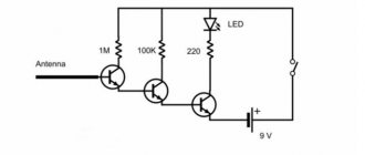
Homemade driver for LEDs from a 220V network
Measuring elements are used when working with metal cable lines. They allow you to neutralize extraneous influences for more efficient localization of defects. Highly accurate results are guaranteed within the range of measured values.
Using a Wheatstone bridge circuit, you can calculate the resistance of a changing element. The circuits are used in the construction of electronic scales, electronic thermometers and thermistors.
Among industrial designs, devices with manual equilibrium calibration are widely known:
- MMV – measures the resistance of a DC voltage conductor;
- P333 is a single bridge circuit, with the help of which a damaged section of the cable is identified.
History of creation
In 1833, Samuel Hunter Christie proposed a scheme that later became known as the Wheatstone Bridge.
In 1843, the scheme was improved by Charles Wheatstone[2] and became known as the “Wheatstone Bridge”.
In 1861, Lord Kelvin used the Wheatstone bridge to measure small resistances.
In 1865, Maxwell measured alternating current using a modified Wheatstone bridge.
In 1926, Alan Blumlein improved the Wheatstone Bridge and patented it. The new device was named after the inventor.
Semiconductor circuits
Any rectifier is a circuit. It includes a secondary winding of the transformer, a rectifying element, an electrical filter and a load. In this case, it is possible to obtain voltage multiplication. Rectified voltage is the sum of DC and AC voltages. A variable component is an undesirable component that is reduced in one way or another. But since half-waves of alternating voltage are used, it cannot be otherwise.
It can be reduced in two ways:
- improving the efficiency of the electrical filter;
- improving the parameters of rectified alternating voltage.
The simplest half-wave rectifier. It cuts off one of the half-waves of alternating voltage. Therefore, the ripple coefficient in such a circuit is the largest. But if a three-phase voltage is rectified with one diode in each phase, as well as the same filter, the ripple factor will be three times lower. However, full-wave rectifiers have the best characteristics.
You can use both half-waves of alternating voltage in two ways:
- according to the bridge diagram;
- according to a circuit with a midpoint of the winding (Mitkevich circuit).
Let's compare both of these circuits for the same value of rectified voltage. The bridge circuit uses fewer turns of the transformer secondary winding, which is an advantage. But at the same time, four diodes are needed in a single-phase rectifier bridge. The midpoint circuit requires twice as many turns of the midpoint secondary winding, which is a disadvantage. Another disadvantage of this scheme is the need for symmetry of the winding parts relative to the midpoint.
Voltage stabilizer circuit diagram
Asymmetry will be an additional source of pulsations. But this circuit only needs two diodes, which is an advantage. When rectifying, there is voltage across the diode. Its value almost does not change depending on the current flowing through this diode. Therefore, the power dissipated by a semiconductor diode increases as the rectified current increases.
This is very noticeable at high current levels, and therefore semiconductor diodes are placed on cooling radiators and, if necessary, are blown.
When rectifying high current, two diodes of a midpoint circuit will be more economical and more compact compared to four diodes of a rectifier bridge. Rectifier circuits did not appear out of nowhere back in the day. They were invented by engineers. Therefore, rectifier circuits in the literature are sometimes named in connection with the names of their discoverers. The bridge circuit is referred to as a “full Graetz bridge”. A circuit with a midpoint is a “Mitkevich rectifier”.
Power transformer
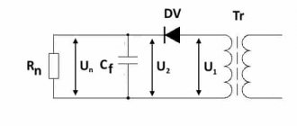
This device is designed to match the voltages at the input and output of the rectifier device. In other words, the transformer separates the load network and the power network. There are various options for connecting the windings of this transformer, the choice of which depends on the type of rectification circuit of the device. The value of the output voltage of transformer U2 is influenced by the voltage value at the output of the rectifier bridge Un.
The transformer is capable of galvanic isolation of frequency f1 from the power supply network U1, I1, and the load circuit from Un, In simultaneously. Currently, it is possible to design and produce high-voltage inverters that operate at higher frequencies and rectify voltage. For this purpose, transformerless rectification schemes are used, in which the valve block is connected directly to the primary power supply network.
Power transformer
Diode bridge
This block performs the main function in the rectifier device, converting alternating current into direct current. The block most often uses elements in the form of diodes. At the output of the valve block, a constant voltage is removed, which has an increased pulse level, which depends on the number of phases of the power supply network and the rectifier circuit.
Diode bridge
Filtration device
The filtering part of the rectifier provides the required level of voltage ripple at the output of the rectifier in accordance with the load requirements. The filter device circuit uses a smoothing choke or resistor connected in series and capacitors connected in parallel with the power output.
However, most often filters are made according to somewhat more complex schemes. In low-power rectifiers there is no need to use a choke and resistor. In rectifier circuits for three-phase networks, the magnitude of the pulses is smaller, thereby making the operating conditions of the filter easier.
Classification
Balanced and unbalanced measuring bridges are widely used in industry.
Work of the Balanced
bridges (the most accurate) is based on the “zero method”.
With the help of the unbalanced
bridges (less accurate), the measured value is determined by the readings of the measuring device.
Measuring bridges are divided into non-automatic and automatic.
In non-automatic
On bridges, balancing is done manually (by the operator).
In automatic
The bridge is balanced using a servo drive based on the magnitude and sign of the voltage between points D and B (see figure).
Measuring bridge circuits
AC measuring bridges are divided into 2 groups: double and single. Single ones have 4 shoulders. In them, 3 branches create a circuit with 4 connection points.
There is an electromagnetic galvanometer in the diagonal of the bridge that shows balance. In the other diagonal of the bridge there is a constant power source. Measurements may have errors depending on their range. As the resistance increases, the sensitivity of the device decreases.
A double bridge is called a six-arm bridge. Its arms are the measured resistance (Rx), a resistor (Ro) and 2 pairs of additional resistors (Rl, R2, R3, R4).
Application for measuring non-electrical quantities
The Wheatstone bridge is often used to measure a wide variety of non-electrical parameters, for example:
- mechanical deformations of elastic elements in strain gauges;
- temperature;
- illumination;
- composition of the substance, including humidity and gas analysis;
- thermal conductivity and heat capacity and much more.
The operating principle of all these devices is based on measuring the resistance of a sensitive resistive element-sensor, the resistance of which changes when the non-electrical quantity acting on it changes. The resistive sensor(s) are electrically connected to one or more arms of the Wheatstone bridge and the measurement of a non-electrical quantity is reduced to measuring the change in the resistance of the sensors.
The use of the Wheatstone bridge in these applications is due to the fact that it allows one to measure a relatively small change in resistance, that is, in cases where Δ R x / R x ≪ 1. {\displaystyle \Delta R_{x}/R_{x}\ll 1.}
Typically, in modern instrumentation, the Wheatstone bridge is connected via an analog-to-digital converter to a digital computing device, such as a microcontroller, that processes the bridge signal. During processing, as a rule, linearization is carried out, scaling with conversion to a numerical value of a non-electrical quantity in units of its measurement, correction of systematic errors of sensors and measuring circuits, indication in a digital and/or machine-graphic form that is convenient and visual for the user. Statistical processing of measurements, harmonic analysis and other types of processing can also be performed.
Operating principle of strain gauges
Main article: Strain gauge
Strain gauges and strain gauges are used in:
- electronic scales;
- dynamometers
- pressure meters (manometers);
- torque meters on shafts (torsiometers);
- measuring the deformation of parts under the influence of mechanical load, etc.
In this case, strain gauges glued to elastic deformable parts are included in the arms of the bridge, and the useful signal is the voltage of the diagonal of the bridge between points D
and
B
(see picture).
If the relation holds:
R 1 / R 2 = R 3 / R x , {\displaystyle R_{1}/R_{2}=R_{3}/R_{x},}
then, regardless of the voltage on the diagonal of the bridge between points A
and
C
(voltage) between points
D
and
B
( UDB {\displaystyle U_{DB}} )) will be equal to zero:
UDB = 0. {\displaystyle U_{DB}=0.}
But if R 1 / R 2 ≠ R 3 / R x , {\displaystyle R_{1}/R_{2}\neq R_{3}/R_{x},} then a non-zero voltage (“imbalance” of the bridge) will appear on the diagonal, uniquely associated with a change in the resistance of the strain gauge, and, accordingly, with the amount of deformation of the elastic element, when measuring the imbalance of the bridge, the deformation is measured, and since the deformation is associated, for example, in the case of scales, with the weight of the body being weighed, its weight is measured as a result.
To measure alternating strains, in addition to strain gauges, piezoelectric sensors are often used. The latter have replaced strain gauges in these applications due to their better technical and operational characteristics. The disadvantage of piezoelectric sensors is that they are not suitable for measuring slow or static deformations.
Measurements of other non-electrical quantities
The described principle of measuring strain using strain gauges in strain gauges is preserved for measuring other non-electrical quantities using other resistive sensors, the resistance of which changes under the influence of a non-electrical quantity.
Temperature measurement
These applications use resistive sensors that are in thermal equilibrium with the body being studied; the resistance of the sensors changes as their temperature changes. Sensors are also used that do not directly contact the body under study, but measure the intensity of thermal radiation from the object, for example, bolometric pyrometers.
As temperature-sensitive sensors, resistors made of metals are usually used - resistance thermometers with a positive temperature coefficient of resistance, or semiconductors - thermistors with a negative temperature coefficient of resistance.
Indirectly through temperature measurement, thermal conductivity, heat capacity, flow rates of gases and liquids in hot-wire anemometers and other non-electrical quantities related to temperature are also measured, for example, the concentration of a component in a gas mixture using thermocatalytic sensors and thermal conductivity sensors in gas chromatography.
Measurement of radiation fluxes
Photometers use sensors that change their resistance depending on the illumination - photoresistors. There are also resistive sensors for measuring ionizing radiation fluxes.
There are two options for using a Wheatstone bridge to measure electrical resistance:
- Determination of the absolute value of resistance by comparison with a known resistance.
- Determination of relative changes in resistance.
The latter option is used in relation to strain gauge measurement methods. It allows you to determine with great accuracy the relative changes in the resistance of the strain gauge in the common range from 10 -4 to 10 -2 Ohm / Ohm.
The image below shows two different illustrations of a Wheatstone bridge: Figure a) is a normal diamond image using a Wheatstone bridge; Figure b) shows an image of the same electrical circuit, but more understandable for a beginner.
The four branches of the bridge circuit are formed by resistances from R 1 to R 4. Corner points 2 and 3 indicate connections for the bridge excitation voltage V s . The bridge output voltage V0, that is, the measurement signal, is available at corner points 1 and 4.
There is no generally accepted rule for naming bridge components and connections. There are all sorts of notations in the popular literature, and this is reflected in the bridge equations. It is therefore important that the designations and indices used in the equations are taken into account along with their position in the bridge circuits, this will help to avoid confusion.
If the supply voltage V s is applied to the bridge supply points 2 and 3, then the supply voltage is divided into two halves of the bridge R 1, R 2 and R 4, R 3 as the ratio of the corresponding bridge resistances. , i.e. each half of the bridge forms a voltage divider.
The bridge may be unbalanced due to differences in voltages and electrical resistances across R 1, R 2 and R 3, R 4. This can be calculated as follows:
if the bridge is balanced and
where the bridge output voltage V 0 is zero.
For a given deformation, the resistance of the strain gauge changes by the amount ΔR. This gives us the following equation:
To measure strain, the resistances R 1 and R 2 in a Wheatstone bridge must be the same. The same applies to R 3 and R 4 .
With a few simplifications, the following equation can be derived:
At the last stage of the calculation, ΔR/R must be replaced by the following:
Here k is the k coefficient of the strain gauge, ε is the deformation. We get the following:
The equations assume that all resistances in the bridge change. Designations such as quarter bridge, half bridge, double quarter or diagonal bridge and full bridge are common.
Although the above-mentioned definitions such as “half-bridge” or “quarter-bridge” are used to designate such circuits, in fact they are not entirely correct. In fact, the circuit used for measurement is always complete and is formed entirely or partially by strain gauges. They are then supplemented by fixed resistors, which are built into the measuring instruments.
Weighing terminals typically meet very stringent accuracy requirements. Therefore, unlike experimental measuring instruments, weighing transducers should always have a full bridge circuit with active load cells on all four arms.
In case it is necessary to eliminate various interferences and factors interfering with the measurement, full-bridge or half-bridge circuits are used for load analysis. An important condition is a clear distinction between stresses and forces, such as compression or tension, as well as bending, shearing or twisting forces.
The table below shows the relationship between the position of the strain gauges, the type of bridge circuit used and the resulting bridge coefficient B for normal forces, bending moments, torque and temperature. The small tables provided for each example indicate the bridge coefficient B for each type of influence quantity. These equations are used to calculate the effective voltage from the output of the VO/VS bridge.
| Bridge configuration | Calculation | Measurement | Description | Advantages and disadvantages | |
| 1 | Measuring strain on a tension/compression bar Measuring strain on a bending beam | Simple quarter bridge Simple quarter bridge circuit with one active load cell | + Easy installation — Normal deformation and bending deformation are superimposed on each other - Temperature effects are not automatically compensated | ||
| 2 | Measuring strain on a tension/compression bar Measuring strain on a bending beam | Quarter Bridge Two quarter bridge circuits, one actively measures deformation, the other is mounted on a passive component made of the same material that does not undergo deformation. | + Temperature effects are well compensated - Normal deformation and bending deformation cannot be separated (flexural superposition) | ||
| 3 | Measuring strain on a tension/compression bar Measuring strain on a bending beam | Poisson half-bridge Two active load cells connected by a half-bridge, one of which is located at a 90° angle to the other | + Temperature effects are well compensated when the material is isotropic | ||
| 4 | Measuring the deformation of a bending beam | Half-bridge Two strain gauges are installed on opposite sides of the structure. | + Temperature effects are well compensated + Separation of normal and bending strain (only the bending effect is measured) | ||
| 5 | Measuring strain on a tension/compression bar | Diagonal bridge Two strain gauges are installed on opposite sides of the structure. | + Normal strain is measured independently of bending strain (bending excluded) | ||
| 6 | Measuring strain on a tension/compression bar Measuring strain on a bending beam | Full bridge 4 load cells are installed on one side of the structure as a full bridge. | + Temperature effects are well compensated + High output signal and excellent common mode rejection (CMR) — Normal deformation and bending deformation cannot be separated (bending superposition) | ||
| 7 | Measuring strain on a tension/compression bar | Diagonal bridge Two active load cells, two passive load cells | + Normal deformation is measured independently of bending deformation (bending excluded) + Temperature effects are well compensated | ||
| 8 | Measuring the deformation of a bending beam | Full Bridge Four active load cells connected as a full bridge | + Separation of normal and bending deformation (only the bending effect is measured) + High output signal and excellent common mode rejection (CMR) + Temperature effects are well compensated | ||
| 9 | Measuring strain on a tension/compression bar | Full bridge Four active load cells, two of which are rotated 90° | + Normal strain is measured independently of bending strain (bending excluded) + Temperature effects are well compensated + High output signal and excellent common mode rejection (CMR) | ||
| 10 | Measuring the deformation of a bending beam | Full bridge Four active load cells, two of which are rotated 90° | + Separation of normal and bending deformation (only the bending effect is measured) + High output signal and excellent common mode rejection (CMR) + Temperature effects are well compensated | ||
| 11 | Measuring the deformation of a bending beam | Full bridge Four active load cells, two of which are rotated 90° | + Separation of normal and bending deformation (only the bending effect is measured) + High output signal and excellent common mode rejection (CMR) + Temperature effects are well compensated | ||
| 12 | Measuring the deformation of a bending beam | Full Bridge Four active load cells connected as a full bridge | + Separation of normal and bending deformation (only the bending effect is measured) + Temperature effects are well compensated + High output signal and excellent common mode rejection (CMR) | ||
| 13 | Measuring torsional strain | Full Bridge Four load cells are installed, each at an angle of 45° to the main axis, as shown. | + High output signal and excellent common mode rejection (CMR) + Temperature effects are well compensated | ||
| 14 | Measuring torsional strain in limited installation space | Full Bridge Four load cells are mounted as a full bridge at a 45° angle and overlap each other (rosettes) | + High output signal and excellent common mode rejection (CMR) + Temperature effects are well compensated | ||
| 15 | Measuring torsional strain in limited installation space | Full Bridge Four load cells are mounted as a full bridge at a 45° angle and overlap each other (rosettes) | + High output signal and excellent common mode rejection (CMR) + Temperature effects are well compensated | ||
Examples 13, 14 and 15 assume a cylindrical shaft to measure torque. For reasons of symmetry, bending in the X and Y directions is allowed. The same conditions apply for bars with a square or rectangular cross-section.
Explanation of symbols:
| T | Temperature |
| Fn | Normal strength |
| M b | Bending moment |
| M bx , M - by user | Bending moment for X and Y directions |
| M d | Torque |
| εs | Apparent voltage |
| ε n | Normal voltage |
| ε b | Bending deformation |
| ε d | Torsional deformity |
| ε | Effective strain at the measuring point |
| ν | Poisson's ratio |
| Active load cell | |
| Load cell for temperature compensation | |
| Resistor or passive strain gauge |
Modifications
Using a Wheatstone bridge, resistance can be measured with great accuracy.
Various modifications of the Wheatstone bridge make it possible to measure other physical quantities:
- capacity;
- inductance;
- impedance;
- gas concentration;
- and other.
The explosimeter device allows you to determine whether the permissible concentration of flammable gases in the air is exceeded.
The Kelvin bridge, also known as the Thomson bridge, allows the measurement of small resistances, invented by Thomson.
Front view of a device based on the Kelvin bridge
The Maxwell device allows you to measure the strength of alternating current, invented by Maxwell in 1865, improved by Blumlein around 1926.
The Maxwell bridge allows you to measure inductance.
The Carey Foster bridge allows the measurement of small resistances, described by Carey Foster in a document published in 1872.
The Kelvin-Varley voltage divider is based on a Wheatstone bridge.