Anyone who wants to deepen their skills in repairing, servicing electrical equipment, and performing diagnostic activities needs to know how to use an oscilloscope. An oscilloscope is designed to monitor voltage changes over time. The device is equipped with a moving scan screen showing graphs, amplitude, and sinusoidal oscillations for certain periods.
What is an oscilloscope
An oscilloscope (O-Scope, Oscilloscope) records changes (amplitudes, fluctuations) in the voltages of electrical circuit signals with output in the form of sinusoids, sawtooths and other lines on a coordinate grid on the monitor. The device is used to study the dynamics of a system during its operation. A typical example: testing pulsed, generator devices (power supplies). The oscilloscope will show the shape of voltage, electrical signals over time, the level of fluctuations, changes under certain conditions and factors (breakdowns, temperature, magnetic fields, interference, shielding).
Purpose
O-Scope measures these quantities and solves the following problems:
- test measures for electrical circuits, assemblies, products during their production, repair, in research institutions;
- always used when testing measuring devices;
- electrical, television and radio sphere: properties of signals, degree of noise, distortion;
- for highly specialized hardware, for analyzing automated control systems, executive devices;
- measurements of frequencies and amplitudes during debugging;
- visual monitoring of signals, phase shifts;
- analysis of the functioning of vehicle sensors.
Briefly displaying the functions, the device allows you to observe voltage changes:
- in time: frequency, intervals, duty cycle, cycles, jumps, recessions, bursts;
- in physics: vibrations, amplitudes, max./min. RMS values.
An oscilloscope is the “eye” that allows you to look inside a circuit as it operates. In addition to simple measurement of an electrical signal, modern products can perform mathematical transformations in real time (Fourier, etc.).
Where is it used?
Areas of application:
- always in scientific, technical laboratories, research departments at factories that produce electrical appliances, for example, the manufacturer must know how his products react to interference;
- during in-depth analysis of assemblies, during adjustment and repair of electrical devices: from radio and cellular communications to machine motor circuits. The device is indispensable for radio amateurs.
The device provides visual information about the characteristics of complex signals, shows time and amplitude data of changes, which is important for calculations and determining how the studied object will behave over periods under specific conditions.
What can an oscilloscope measure?
An oscilloscope can measure:
- will show by signals: shape;
- frequency;
- period;
- amplitude;
- phase shift angle;
- comparison of signals;
O-Scope is actually a voltmeter, but it displays online voltage changes; it can be used to indicate the shape of the current by connecting a resistor in series to the network being served (Rt, “t” - current, also shunting). Its Ohm number is selected much lower than that of the circuit so that there is no influence on the circuit. Next, it is calculated using the formula and, knowing the value of Rt, you can find the current.
Oscilloscope sensitivity
The peculiarity of the photocapacitance method is to measure small changes in capacitance under the influence of illumination with large capacitances of the structure and input capacitances of the measuring circuit.
The actual sensitivity is determined by both the sensitivity of the measuring circuit and the stability of the current-voltage characteristic of the structure under study. The minimum change in AC/C capacitance when using bridge measurement methods is approximately 10~3. Therefore, the minimum concentration of depth- The sensitivity of deflection systems is the ratio of the displacement of the electron beam on the working surface of the electron receiver to the value of the deflection factor that caused it. For tubes with electrostatic deflection, sensitivity is determined by the ratio of the displacement h [mm] of the luminous spot on its screen to the deflecting voltage ?/control [V]:
Since when converting mechanical stresses, the initial parameters of magnetoelastic sensors are usually compensated and the decisive role is played not by the relative change in magnetic permeability, but by its absolute increment, the magnetoelastic properties of a material are often characterized by the ratio of the absolute change in magnetic permeability to the relative deformation, and the magnetoelastic sensitivity is defined as
The sensitivity S of an electrical measuring instrument to the measured value x is the derivative of the movement of the pointer along the measured value x. A wide range of electrical measuring instruments use angular movement of the pointer. For these devices, sensitivity is defined as the derivative of the angle of deflection a of the pointer with respect to the value x, i.e.
Sensitivity is one of the most important parameters of any photovoltaic device. For photoresistors, the current sensitivity si is most often used - the ratio of the photocurrent to a certain value that quantitatively characterizes the radiation that caused the measured photocurrent1. So, if the luminous flux is used as such a quantity, then they talk about the sensitivity of the photoresistor to light because s
The integral sensitivity is determined by the ratio of the photodiode current to the luminous flux /Sivt=/f/F.
Generally speaking, the sensitivity of a photodetector is not a constant value and depends, in particular, on the radiation parameters. To take this dependence into account, the concepts of static and dynamic differential sensitivity of the photodetector are introduced, while the static sensitivity is determined by the ratio of the constant values of the measured quantities. Expression (5.34), for example, allows you to determine the value of the corresponding static sensitivity. Differential sensitivity is equal to the ratio of small increments of measured quantities: for example, the differential current sensitivity of a photodetector to illumination
Mathematically, sensitivity is determined by the formula
Sensitivity is one of the most important parameters of any photovoltaic device. For photoresistors, the current sensitivity si is most often used - the ratio of the photocurrent to a certain value that quantitatively characterizes the radiation that caused the measured photocurrent1. So, if the luminous flux is used as such a quantity, then they talk about the sensitivity of the photoresistor to light because s
Having the transformation equation, you can find an expression for one of the most important parameters of measuring instruments - the absolute sensitivity S, which in the general case is S = dY/dX. For a linear transformation equation, sensitivity is determined by the slope of the straight line (3.1):
The sensitivity S of an electrical measuring device to the measured value x is the derivative of the position of the pointer with respect to the measured value x. A wide range of electrical measuring instruments use angular movement of the pointer. For these devices, sensitivity is defined as the derivative of the deflection angle a of the moving part with respect to x, i.e.
The sensitivity of an oscilloscope is the ratio of the vertical deviation of the light spot on the screen in millimeters to the value of the input voltage in volts. The sensitivity of the tube itself, without an amplifier, is relatively low, approximately 0.5-1 mm/V. However, the use of gain increases the sensitivity of the oscilloscope to 1 - 2 mm/mV.
The value of Sy, depending on the transmission coefficients D and Vs. V and on the sensitivity of the tube are called the sensitivity of the oscilloscope at the V input.
The sensitivity of an oscilloscope is the ratio of the vertical deviation of the light spot on the screen in millimeters to the value of the input voltage in volts. The sensitivity of the tube itself, without an amplifier, is relatively low, approximately 0.5-1 mm/V. However, the use of amplification increases the sensitivity of the oscilloscope to 1-2 mm/mV.
When plate x - x is supplied with a sinusoidal voltage t, then it is possible to measure the frequency / of the input voltage, sinusoidal and the frequency is a multiple of the frequency fx. Depending on the frequency ratio /// there are different figures on the oscilloscope screen (12.31). The sensitivity of an oscilloscope is the ratio of the vertical deviation of the light spot on the screen in millimeters to the voltage value in volts. The sensitivity of the tube itself is relatively low, approximately 0.5-1 mm/V. However, the example increases the sensitivity of the oscilloscope to 1 -
where ? is the sensitivity of the oscilloscope along the Y axis, mV/mm; Kpzt is the conversion coefficient of the measuring transducer, determined together with the matching amplifier during calibration, mV/g (voltage and acceleration in amplitude values).
The use of amplifiers increases the sensitivity of the oscilloscope to voltage to values of approximately units and tens of centimeters per volt. It should be borne in mind that the gain of the UVO is usually much greater than the gain of the GO. This is explained by the fact that the voltage level created in the GR is quite high and its significant amplification is not required.
When using an oscilloscope as a peak-to-peak voltmeter, the measured AC voltage is applied to the Y channel input, usually with the sweep generator turned off. In this case, the electron beam will draw a vertical straight line on the screen, the length of which, with a sinusoidal measured voltage, will be proportional to its double amplitude: /V = 8u-2it. Knowing the sensitivity 8i or the beam deflection coefficient k0, we can find
The value of the Zc or k0 value can be determined by the position of the “Sensitivity” knob on the oscilloscope or by preliminary calibration using an amplitude calibrator. If it is necessary to evaluate the shape of the voltage under study, the scan generator is turned on.
Voltage sensitivity of the oscilloscope is no less than 0.12 lsh/epost;. by current - no less than 120, 12, 2.3 zl/apost.
The use of amplifiers increases the sensitivity of the oscilloscope to voltage to values on the order of units and tens of centimeters per volt. It should also be borne in mind that the gain of the vertical deflection is usually much greater than the gain of the horizontal deflection amplifier. This is explained by the fact that the amplitude of the voltage created by the scan generator is quite large, therefore, in most cases, a significant increase in this voltage is not required. It should be noted that in the literature, as well as in GOST (for example, GOST 9810-61), the term “deviation coefficient” is often used, which is understood as the magnitude, inverse of sensitivity, i.e. the ratio of the input voltage of the oscilloscope in volts or millivolts to the voltage caused by it beam deviation by 1 cm.
The cillographic tube must have the highest possible sensitivity for deflection in order to provide the necessary sensitivity of the oscilloscope while the amplifier gain is not too high. :
Kinds
Digital models have recording and archiving functions, which expands the possibilities. To compare results online, devices with several channels are used. There are copies connected to a PC and combinations with other measuring devices.
The choice of analog models (except for simple and educational ones) implies knowledge of a variety of settings, the adjustment is complicated. On the other hand, such devices provide in-depth practice.
Digital models are the recommended choice and will allow you to quickly learn the basics. These are computing systems, with them data acquisition and interpretation are easier and much faster. There are also analog-digital models.
Operating principle of a digital oscilloscope
Digital oscilloscopes, unlike analog ones, do not repeat the received signal directly to the screen, but first convert it into “digital” form. To do this, the input signal is measured a certain number of times per second, then the device, after some transformations of this data, reconstructs the signal and displays it on the screen. Digitization is performed using an analog-to-digital conversion unit.
Device
The main unit of the oscilloscope is a tube like in old TVs, a cathode-ray tube that visualizes the quantities received by the input divider, on which the scope of permissible measurements depends. Amplification occurs and synchronization with the scan generator occurs. Next, the value under study reaches the final amplifying node, the CRT, and then it is displayed online without any delays.
The algorithm for how a digital oscilloscope works is somewhat different: it first passes the signal through a converter (analog-to-digital), measuring it several times per second. Then reconstruction and display on the monitor occurs. At the same time, the data is recorded in the buffer memory, and there is the possibility of future processing.
It is more convenient to work with a digital oscilloscope; its advantages are full functionality with additional options in a small case, ease of settings. The choice of an oscilloscope in modern conditions is usually made among the specified types. Some analog old solid Soviet copies (4–5 times cheaper) are not bad, but they are bulky and require more setup skills.
Applications and measurement methods
Oscilloscopes are used in many areas of industry. They are used to diagnose power supplies, converters, when repairing mobile phones, on television to adjust the incoming signal, when developing electrical equipment, etc. When considering the principles of operation of an oscilloscope, it is important to study measurement techniques. There are 4 of them in total:
- Voltage measurement. The procedure is carried out in linear scan mode. The generator is connected to the device being measured. Usually one of the connection points acts as a “ground”, but this rule is not mandatory. Voltage values are measured from peak to peak. Once the voltage is obtained, other parameters can be determined using simple calculations.
- Measurement of time and frequency. For this procedure, the horizontal scale of the device is used. The device measures the duration and period of the pulses, and the frequency is the reciprocal of the period.
- Measurement of pulse duration and rising edge duration. Distorted pulses are one of the common causes of electrical circuits not working properly. To run this measurement algorithm, you must fine-tune the device. It is especially important to correctly use the trigger hold mode and the horizontal stretch function (to view small details of short pulses).
- Phase shift measurement. The device analyzes the timing difference between two identical signals. One signal is sent to the device's vertical deflection system, and the second to the device's horizontal deflection system.
We should not forget about other measuring technologies used in modern types of equipment. With their help, you can configure the device to capture fast processes in production, test electronic components, etc.
How an oscilloscope works
If you look at quickly passing objects, you will see a blurry line. But if you periodically open the “window”, static frames will be captured. This is the principle of a strobe, the same, but in electronic form the Oscilloscope works.
The action of the “window” is synchronized (the main condition) with the speed of the objects (signal), so when it opens, their place is stable. Otherwise, desynchronization will occur.
The device visualizes periodic changes in real time on the display using a sinusoid or a line of another shape (saw, meander, etc.). Each future segment is similar to the past, it “stops” and is shown (at 1 moment - 1 period).
Types of oscilloscopes and their applications
Oscilloscopes are one of the most common types of instrumentation, along with multimeters, providing scientific and industrial research.
There are several types of oscilloscopes, differing both in characteristics and operating principles. The first type is analog oscilloscopes.
These devices are the most common representatives of this type of measuring devices and have occupied a key place in the market for a long time. Any analog oscilloscope, regardless of its characteristics, consists of several main components: - Input signal divider;
— Amplifier of deviations of the vertical plane;
— Scheme of synchronization and deviation of the horizontal plane;
- Power unit;
— Analog output device.
Although digital oscilloscopes are much more advanced and are beginning to replace analog oscilloscopes, the latter stand out due to several key advantages. Thus, the price of analog instruments remains significantly lower, and technological developments have allowed real-time analog oscilloscopes to gain a number of advanced capabilities.
The second type is digital devices. Digital storage oscilloscopes initially offer great opportunities for conducting research, and the relatively high price is compensated by the constant reduction in the cost of digital circuits on the market and, as a consequence, the reduction in cost of the devices themselves.
Any digital oscilloscope consists of the following main components:
— Input signal divider;
— Normalization amplifier;
— Analog-to-digital converter;
- Memory device;
— Information input and output device.
The key advantage of digital storage oscilloscopes is their analysis capabilities: depending on the specified settings, the instrument is able to record readings converted into digital format after normalization. In addition, due to the digitization of the signal, the image is output more stable, and the final result can be recorded and edited in accordance with the requirements (marking, scaling). In addition, the digital output device allows you to display a graphical interface on top of the output information.
The third type of oscilloscopes is digital phosphor devices. Devices of this type operate using digital phosphor technology, which sets their construction methods apart from other types of devices. Today, the price of these devices remains the highest in their class, but the functionality of digital phosphor oscilloscopes allows you to get all the main advantages of both analog and digital devices. Thus, in addition to recording the studies performed, digital phosphor oscilloscopes are able to simulate changes in the intensity of the output image, which allows the operator to display all the fine details of the modulated signals.
The fourth type is virtual oscilloscopes. Virtual instruments are a relatively new type of device designed as an extension to a personal computer. Virtual oscilloscopes are capable of operating both through the common USB interface and through PCI and ISA interfaces, providing flexible options for installing the device. In addition, the software of virtual oscilloscopes allows you to interact with the computer operating system at the native level, ensuring data collection and processing by the computer's computing power, which allows you to achieve greater capabilities for grouping and analyzing information.
Digital oscilloscopes have relatively small dimensions, high performance and low cost, which makes this class very competitive.
The fifth type is portable devices. Portable oscilloscopes emerged as a consequence of the development of digital technology and the widespread reduction of digital circuits. Thus, according to the characteristics of the research carried out, portable oscilloscopes are the same as stationary devices, but with improved weight-dimensional properties and the ability to operate autonomously.
What to look for in an Oscilloscope, guidelines for selection
Let's look at the basic characteristics of O-Scope, which will also serve as guidelines on how to choose an oscilloscope and its reliable model.
Ways to check the oscilloscope:
- built-in generator (Calibration), all digital models have it. Turn on the mode and see if there is a sinusoid. If the store is specialized, there should be an external generator for testing;
- old oscilloscopes begin to change over time, there is a simple way to check them: take a reference source, for example, the same 1.5 V battery;
- the screen must be of sufficient brightness, the beam must be free of artifacts;
- touch the probe: the phase will show a sinusoid (though with a lot of noise), the ground will show a flat line;
- via PC, special software.
Bandwidth
These are the minimum and maximum frequencies, amplitude, that is, the range that the device can measure. It is enough to take into account the top line; the bottom one is drawn by all devices.
Sampling rate
For digital models. This parameter is related to the previous one. The higher the better (for example, Siglent SDS has 1×10⁹). This number of readings per unit time determines the maximum frequencies without loss on the screen. For devices with several channels, it may decrease when all of them are used (must be taken into account when purchasing).
According to Kotelnikov's theorem, part. disc. should exceed the upper transmission frame by 2 times, but in practice an excess of 4–5 times will be required. This is what the choice is based on. Example for a product with a bandwidth of up to 200–800 MHz (it is important to take into account this parameter when using 2 or more channels).
Number of channels
Many models are capable of processing more signals together while simultaneously displaying them separately on the monitor. Usually from 2 to 4. Sometimes turning on other channels affects performance. It is recommended to choose an oscilloscope among products with two channels, which will allow you to compare the quantities under study and calculate phase shifts. Three or more inputs are good, but for ordinary tasks it is sometimes excessive, the price of the device will increase many times over.
Equivalent sampling rate
When the real part is not enough. discrete, the final image is reconstructed from several successive measurements. Example: a 200 MHz signal is analyzed on a model with a frequency. disc. 1 billion samples/sec. (1 GSa/s) - only 5 measurements are obtained. According to theory This is enough for Kotelnikov, but you can detail it (algorithmically) and activate the option: there will be not 1 GSa/s, but 2 GSa/s.
Memory depth
Always available in digital models (DSO=Digital Storage Oscilloscope). The lower the sweep speed, the more accurate the readings and the more values the device has to store in memory. The deeper the memory, the better. But sometimes there is a negative point: during slow measurements, the device slows down; when choosing a product, you need to inquire about this nuance.
Screen update
The more often the monitor is updated, the shorter the “dead time” required to process the captured information, and the more quickly the waveforms are updated. There is a greater chance that the device will show a subtle artifact. However, this only matters for electronics fans.
Maximum input voltage (supply)
Any device has a limit on power supply, if it is exceeded without additional measures it will simply burn out and fail. It is necessary to take into account the parameters of the serviced circuits. Example: max. eg in the probe mode 1:1 - 40 V, in the 1:10 mode - 400 V, that is, it is no longer safe to climb into a circuit with 400 V or more without safety measures.
Beginning of work
Working with an oscilloscope using an analog device is described in more detail. As an object of study, you can use simple models: an extremely simple educational oscilloscope n3013 or the popular S1-83. Digitally everything is the same, but it unifies and generalizes some points.
In the Oscilloscope beam tube, beams of electrons going to the display provoke the glow of the phosphor (light dot in the middle). Deflection plates (2 pairs) make it possible to drive it. The higher the voltage at the terminals, the more it moves. The applied stress to the formation. X (vertical) initiates a sawtooth scan, the beam runs cyclically (this is the scan or zero line). To the layer Y connect the quantities under study.
Synchronization
Before working with an oscilloscope, you need to learn the basics (control, connections, what probes, etc.). The main point of interaction is synchronization. If the start of the saw (the leftmost position of the beam) and the signal coincide, then 1 scan pass will show 1 or more periods and the image will seem to freeze. Changing speed sweeps make it so that there will be only 1 segment on the scoreboard: for 1 lane. saws will pass 1 lane. analyzed signal.
Synchronization methods:
- The saw and the signal are synchronized, adjusting the speed with the selector until the sinusoid stops
- The level is set, the input voltage is indicated to activate the generator. The saw will appear only when the value is set, synchronization is automatic. It is necessary to take into account interference: it can activate the generator erroneously (the level is too low), if it is very high, the signal will not start the system.
You need to know the following:
- the horizontal displacement of the beam is directly proportional to time;
- vertically - proportional to the voltage being tested.
Connection
An oscilloscope does not have two separate probes, like a multimeter. There is one cable with 2 branches, conductors (voltage is measured between 2 points), plugged into a socket with 2 terminals. If the device has more than one socket with them, then the device is two or multi-channel.
Two terminals:
- for phase - connected to the input of an amplifier that deflects the beam vertically;
- common (ground, minus) - connected directly to the device body.
In foreign devices, the wire with the “crocodile” is the ground, the phase is a needle, which is poked into the contacts of the circuits being tested, into the legs of microprocessors, etc. In domestic products, the wires are often the same. You can find out the purpose by touching them with your hand: minus (ground) - there is a straight line on the screen, phase - a distorted sinusoid.
You cannot use any probe wire - in an oscilloscope these are only coaxial special products, any other cable will show nonsense.
A simplified algorithm of use, how to connect to the analyzed circuit and conduct research:
- The oscilloscope is placed in a convenient place, the handles are brought to the normal or neutral position.
- If you have a calibrator, you need to calibrate it according to the instructions.
- The earth is planted on the “−” or common core in the circuit under study. If they cannot be determined, they are connected to any of the contacts between which the study is being conducted. The signal is poked according to the scheme.
The device displays the voltage on the probe in relation to the general wiring. Some of these cords (directly on them) have dividers 1:0, 1:100 with on/off toggle switches, allowing you to plug the ends directly into 220 V without risking burning the device.
Input mode
The regulator with a straight line and, below it, a wavy line is the input mode. Upper position - it is permissible to apply any voltage. Medium—allows you to set the scan. The lower position is only for a variable value, and the connection is made through the built-in capacitor.
Example: it is necessary to analyze the interference on a power supply with 12 V, its intensity can be up to 0.3 V. It is not noticeable against a background of 12 V. You can increase the coefficient. along Y, but the graph will go beyond the monitor, and the offset will not be enough to observe the vertex. Then we include a capacitor in the circuit and 12 V will settle there, and a variable value will go into the O-Scope - 0.3 V of interference, the visualization will be enhanced and the full scale will be examined.
Fast start
The screen is marked with lines with divisions Y (vertical) and X (horizontal) - this is a Cartesian coordinate system, their selectors (large and noticeable) are the main controls:
- Gain (V/div, volts/div) - Scales the Y axis to view the entire signal, and also tells you how many volts per division will ultimately be displayed. Example: if there is 2 V per division, and the signal occupies two cells in height, then the amplitude is 4 V; when selecting 1 V and supplying a sinusoid ampl. at 0.2 V it will take 4 cells;
- Duration (Sweep) - frequency adjustment. Here the divisions are in ms and μs. The smaller the gap and the greater the frequency, the higher the high-frequency signal can be seen and by its width you can calculate how many cells it is, and multiplying by the scale. along line X, we get its duration in seconds. You can calculate one period, then the frequency value - f=1/t. This knob is for setting the beam speed on the display left/right. In digital devices there is a solid line. The signal arriving through the input deflects the beam up/down: a wave-like sine wave, saw or other line shape appears, displaying noise and interference.
The expand key and the arrow keys will allow you to move the graph across the screen for ease of perception and to adjust the desired area to the grid squares. And by changing the speed and frequency of the beam (sweep frequency), we achieve synchronization and freezing of the image.
Instructions for the oscilloscope
The printed circuit board has dimensions of 116 x 76 x 19 mm and a weight of 84 g.
A probe with a BNC connector ends with a pair of alligator clips, its length is 50 cm. The oscilloscope board has a 2.4-inch diagonal color screen. At the top of the board there is a high-frequency connector for supplying the signal under study and a 9 V power connector.
At 8.2 V, the oscilloscope draws 100 mA current. The design of the device provides a miniUSB port, but the oscilloscope cannot receive power through it.
When power is applied, information about the device type is displayed on the oscilloscope screen, as well as a warning.
Then the device goes into operating mode.
To test the device, a signal generator of variable frequency and duty cycle was used [1]. To the right of the screen are the operating mode switches. CPL – controls whether the oscilloscope will display all signal components (DC mode) [2-4],
either only the alternating component of the signal (AC), or the oscilloscope input will be grounded (GND).
Switch SEN1 is responsible for the vertical scale. In its different positions, the scale of one vertical coordinate unit is, respectively, 10 mV, 0.1 V or 1V. SEN2 – vertical scale multiplier (X5, X2, X1), by which the voltage value set by SEN1 should be multiplied. Below the screen there is a RESET button to reset the oscilloscope. Next to this button is a green LED that flashes whenever synchronization is triggered.
To the right of the screen there are four control buttons SEL - calling and moving through the settings; “+” and “-” – change the parameter values, OK – confirm the selection.
Naturally, this oscilloscope cannot be compared in functionality to more advanced and expensive models. The maximum signal frequency with which the oscilloscope operates is 200 kHz [2], or even an order of magnitude lower [3], which is very little, but acceptable considering the size and cost of the oscilloscope. The maximum amplitude of the input signal is 50 V [2]. In general, adjusted for cost, the device leaves a favorable impression [4-5]. This oscilloscope can be a portable mini oscilloscope for those who need to perform work outside of an equipped workshop or be the first oscilloscope for a beginner radio enthusiast. Another example of using an oscilloscope is connecting a solar panel to its input. In this mode, it is easy to record pulsations of the light flux from a cheap LED lamp.
Useful: Water turbidity meter: sensor connection diagram and test
In its current version, it is quite difficult to use an oscilloscope. Touching individual contact surfaces on the board with your fingers will distort the readings. In addition, you only need to carelessly place the oscilloscope on a metal object once and after a short circuit you can order a new device.
Measuring voltage
To reduce errors, since observation is visual, it is recommended that the graph occupy 80–90% of the monitor. When measuring voltage and frequency (there is a time interval), it is necessary to place the gain and sweep speed controls in the extreme right positions.
Procedure
Voltage is measured by vertical scaling. Algorithm:
- Before starting, connect the probe signal to its own ground wire (needle to “crocodile”) or set the input mode toggle switch to the “ground” position.
- The “pulse of a corpse” will be displayed, if not, then you need to move the offset, stabilization and level - perhaps the image was hidden and did not start.
- We use the selectors to adjust the shift of the strip to zero and use the “up-down” regulator to set the scan to the horizontal grid, so it will be possible to correctly calculate the height of the oscillogram. If the oscilloscope is old or analog, then you need to let it warm up for about 5 minutes.
- We set the voltage measurement limit, it is recommended to take it with a reserve, then you can reduce it.
- A signal is given to the input (or its switch is moved to one of the operating positions). A graph will appear on the monitor.
- Let's illustrate the process: the battery has 1.5 V, if you touch the ground branch of the probe to its minus, and the signal branch to the plus, then a graph jump of 1.5 Volts will appear.
To find the height of the graph, move the oscillogram with the selector so that the mark by which the amplitude is calculated is on the central vertical with fractions. We get the sensitivity of the deviation - 1 v/div, the size of the oscilloscope. - 2.6 div., and hence ampl. = 2.6 V.
Below is an illustration on an analog device: 3.4 div. — max. voltage. The next picture shows vertical scaling. The “smooth” regulator (the part with the green mark) is in the right limit position, the sensitivity toggle switch is 0.5 V/div. Scale multiplier — ×10. Voltage calculation:
Frequency measurement
Frequency is a time characteristic, intervals, periods of a signal; their measurement is the direct purpose of the oscilloscope. The value under study is always inversely proportional to its period, which can be measured in any area of the oscillogram. But it is more convenient and more accurate to do this at the points where the graph intersects the horizontal line in the center (time axis).
Before the study, set the scan strip to the central horizontal line. Using a handle with an arrow in both directions, we shift the beginning of the period with the leftmost strip on the monitor. In our case, the gap = 6.8 div., speed. sweep - 100 μs/div. Calculations:
Above, two similar pictures show the same signals, but at different scan rates. According to the first image, the frequency calculation (the exact value is 1.459 kHz) has a large error, while according to the second, it is smaller, since greater measurement accuracy is obtained by stretching the image.
In the second figure, the period is slightly greater than 6.8 cases. and the frequency in reality is slightly lower (1.459 KHz) than the received one (1.47 KHz). The deviation is less than 1%, this is acceptable and is considered high accuracy; it will be provided by a digital O-Scope (with linear scan). In analog models the deviation would be higher. A characteristic pattern: as the period increases, the frequency decreases (the proportion is inverse), and vice versa.
Main settings
When considering the principle of operation of an oscilloscope, it is imperative to mention its characteristics. Equipment parameters are extremely important for studying signals. Main characteristics of the measuring device:
- Bandwidth. This is the operating frequency range in which the frequency response decline does not exceed 3 dB relative to the reference frequency. At the reference frequency there is no drop in frequency response.
- Uneven amplitude-frequency response (AFC).
- Nonlinearity of amplitude characteristics of amplifiers.
- Output parameters. The resistance with the input capacitance must be indicated.
- Waveform, i.e. sine wave, sawtooth, square wave, single overshoot, etc.
- Pulse duration or width. Denoted in ms or μs.
The characteristics of faulty equipment being inspected always differ from those indicated in the manufacturer's passport. It is this feature of electrical signals that allows you to quickly diagnose a problem using an oscilloscope.
We measure the phase shift
Sometimes it happens that the phases of voltage and current diverge (when passing through capacitors, inductance). With a two-channel O-scope it is possible to see the level of differences.
The phase shift will show two processes in motion, their position with fluctuations. Not measured in units. time (horizontal), and in fractions of the signal interval (unit of angle). The same relative position of the signals corresponds to the same shift, and it does not depend on the period and frequency. Therefore, measurements are more reliable when the periods on the monitor are stretched to the maximum.
Procedure
Stages (model C1-83):
- Using the arrows of 2 channels (vertically), the scan is set to the center line (there is no signal at the input).
- Gain (vertical) on the first channel they set (steps and smoothly) a larger amplitude, on the second they make it smaller.
- Speed development set up so that 1 specific period fits on the scoreboard.
- The synchronization level is used to set the start of the graph from the time line (sweep, point A), and the selector with a horizontal bar with two arrows is set to start from the extreme left edge of the screen (point A);
- Speed development (steps and smoothly) achieve the finish of the graph on the rightmost vertical edge.
- Repeat the above, stretching the diagram across the entire monitor, the starting and finishing points should coincide with the scan bar.
- The advance is determined, the shift angle (φ) depends on this. Below in the first figure, the current lags behind its start later (ie A and B). In the adjacent figure (b) he is the first, his start is not shown, so they look at the finish of the first half-period: the diagram that started earlier will be the first to reach 0 (mark D approaches faster than B).
φ — angle module, the interval between the starting and finishing points of the period. Next, we find out φ by the rule: 1 interval of any oscillation = 360° (this is a stable proportion).
Measurements are also possible at the ends of periods (D and E), but in the right segment of the monitor the linearity is poor, and the likelihood of errors increases.
Calculus example with graphical illustration: