Oscilloscope: what is it, what are they, what does it measure, how to use

What is an oscilloscope

An oscilloscope is a device for visually displaying and measuring the parameters of signals of various shapes (the process is called “oscillography”). Signals are sent to the input and displayed on the screen. The screen is divided into squares, with two coordinate axes running through the center. Time is measured horizontally. Vertical - amplitude and/or voltage. The division value is set using the calibration knobs. The display mode is adjusted to each signal. Select the mode that is most convenient in this case (within the capabilities of the device).

An oscilloscope is not necessarily a big, bulky thing. There are portable digital models, there are set-top boxes. There are even programs that can be installed on a desktop computer or laptop with an adapter.

This is what a Tektronix DPO 3054 digital oscilloscope looks like. The signal is displayed on the display, the parameters are selected using the controls

Based on the number of simultaneously monitored signals, oscilloscopes are single-beam (single-channel/mono-channel) and multi-beam (multi-channel). Single-beam can receive only one signal at a time, multi-beam - two, three, four or more - up to 16. Depends on the device.

Which type is better? Multibeam. You can simultaneously monitor a signal at several points in the circuit. By changing the parameters, you will see the device’s response not only at the output, but also at different points in the circuit.

Verification methods

Chip testing is a difficult, sometimes impossible process. It's all about the complexity of the microcircuit, which consists of a huge number of different elements.

There are three main ways to check a microcircuit without desoldering, with or without a multimeter:

External inspection of the microcircuit. If you look at it carefully and examine each element, it is possible that you will be able to find some visible defect. This could be, for example, a burnt-out contact (perhaps more than one). Also, when conducting an external inspection of the microcircuit, you can detect a crack in the housing. With this method of checking the microcircuit, there is no need to use a special multimeter device. If defects are visible to the naked eye, you can do without devices.
Checking the microcircuit using a multimeter. If the cause of the part failure is a short circuit, you can solve the problem by replacing the battery.
Detection of violations in the operation of outputs. If a microcircuit has not one, but several outputs at once, and if at least one of them works incorrectly or does not work at all, then this will affect the performance of the entire microcircuit.

Of course, the easiest way to check a microcircuit is the first of those described above: that is, inspecting the part. To do this, just look carefully first at one side of it, and then at the other, and try to notice any defects. The most difficult way is to check with a multimeter.

The influence of the variety of microcircuits

The complexity of verification largely depends not only on the method, but also on the schemes themselves. After all, these parts of electronic computing devices, although they have the same construction principle, are often very different from each other.

For example:

The easiest to check are the circuits belonging to the KR142 series. They have only 3 pins, therefore, as soon as any voltage is applied to one of the inputs, a tester can be used at the output. Immediately after this, you can draw conclusions about performance.
More complex types are “K155″, “K176″. To check them, you have to use a block, as well as a current source with a certain voltage value, which is specially selected for the microcircuit. The essence of the check is the same as in the first option. You just need to apply voltage to the input, and then use a multimeter to check the output values.
If it is necessary to carry out a more complex test - one for which a simple multimeter is no longer suitable, special testers for circuits come to the aid of radio electronics engineers. The method is called ringing the microcircuit with a multimeter tester. Such devices can either be made independently or purchased ready-made. Testers help determine whether a particular circuit node is working. The data obtained during the test is usually displayed on the device screen.

It is important to remember that the voltage supplied to the chip (microcontroller) should not exceed the norm or, conversely, be less than the required level. Preliminary testing can be carried out on a specially prepared test board.

Often, after testing a microcircuit, it is necessary to remove some of its radioelements. In this case, each of the nodes must be checked separately.

Transistor performance

Before checking a radio component with a multimeter, without desoldering, it is necessary to determine which of the two types the transistor belongs to - field-effect or bipolar. If the first, then you can use the following verification method:

Set the device to the “diagnosis” mode, and then use the red probe, connecting it to the element being tested. The other - black - probe should be attached to the collector terminal.
Immediately after completing these simple steps, a number will appear on the device screen that will indicate the breakdown voltage. A similar level can be seen when performing a “ringing” of the electrical circuit between the emitter and the base. It is important not to confuse the probes: the red one should be in contact with the base, and the black one with the emitter.
Next, you can check all the same transistor outputs, but in reverse connection: you will need to swap the red and black probes. If the transistor works well, then the multimeter screen should show the number “1”, which indicates that the resistance in the network is infinitely large.

If the transistor is bipolar, then the probes must be swapped. Of course, the numbers on the device screen in this case will be reversed.

Capacitors, resistors and diodes

The functionality of the microcircuit capacitor is also checked by applying probes to its outputs. In a very short period of time, the value of the resistance shown by the device should increase from several units to infinity. When changing the locations of the probes, the same process should be observed.

To know if a circuit resistor is working, you need to determine its resistance. The value of this characteristic must be greater than zero, but not infinitely large. If, when checking, the device display shows neither zero nor infinity, then the resistor is working correctly.

The process of checking diodes is not particularly complicated. First you need to determine the resistance between the cathode and anode in one sequence, and then, by changing the location of the black and red probes of the device, in another. The health of the diode will be indicated by the tendency of the number displayed on the screen to infinity in one of these two cases and its presence at a mark of several units in the other.

Inductance, thyristor and zener diode

When checking the chip for faults, you may also have to use a multimeter on the current coil . If its wire is broken somewhere, the device will definitely let you know about it. The main thing, of course, is to apply it correctly.

What is it for?

What is an oscilloscope for? This is simply a necessary thing when repairing electronic equipment, when independently assembling or improving any devices. For many people, a tester or multimeter is enough. Yes. But for repairing simple devices without microcircuits and microprocessors. With a multimeter you can check for open circuits, short circuits, and measure voltage and current. Neither the waveform nor the specific parameters of the sine wave or pulses can be measured or seen.

An oscilloscope is needed to measure voltage and visually display signals. The photo shows a Hantek DSO5102B digital two-channel oscilloscope in operating mode

But it happens that all the parts seem to be in good order, but the device does not work. And all because some parts are demanding not only on the physical parameters of the power supply (voltage, current), but also on the signal shape. Some semiconductor parts, almost all microcircuits and processors, suffer from this. And now only the most basic appliances such as a boiler can do without them. So it turns out that you can find a burnt resistor or a broken transistor with a multimeter. But for a slightly more complex breakdown it is no longer possible to eliminate it. It is for these cases that you need an oscilloscope. It allows you to see the waveform, determine if there are any deviations and find the source of the problem.

Checking radio components - part 1

In today's article I would like to touch a little on the topic of electronics and talk about radio-electronic components, or rather about the methodology for testing them.

Professional electricians and even amateurs have to deal with electronics from time to time, so basic knowledge about electronic components will not hurt anyone who deals with electrical work to one degree or another. Since there are currently many radio components, of course I won’t be able to talk about them all, but will only touch on the most common ones. So let's go.

Resistors

Perhaps the simplest and most common radio component is a resistor. A burnt resistor can be easily identified by its blackened, charred body. If the resistor looks normal, you will have to use a multimeter.

To check, set the multimeter to ohmmeter mode. Since the resistor has no polarity, it does not matter which probe is connected to which terminal, it is only important during testing not to touch the current-carrying parts of the probes and resistor terminals with your hands.

We compare the obtained result with the resistor value indicated on the case either in the form of multi-colored stripes or in the form of a numerical value. You can look up the color code for resistors on the Internet or download the program. It is worth noting that a deviation from the nominal resistance of ± 5% is considered quite acceptable.

To check a variable resistor (potentiometer), we measure the resistance between its outer terminals, which should be equal to its nominal value, taking into account the tolerance and measurement error, and also measure the resistance between each of the outer terminals and the middle terminal. The resistance when rotating the potentiometer knob from one extreme position to another should change smoothly, without jumps, from zero to the nominal value.

Capacitors

Along with resistors, capacitors are the most common radio components. On any electronic board you can find various types of capacitors - ceramic, film, electrolytic, etc. Among them, electrolytic capacitors stand out - they are the ones most often susceptible to failure. Probably a classic malfunction that everyone who repaired equipment has encountered is swelling of the capacitor due to overheating, leading to an increase in pressure inside its housing due to evaporation of the electrolyte.

In addition to electrolytes, the same can often be observed with polymer capacitors.

Among the main malfunctions of capacitors, three can be distinguished:

dielectric breakdown that occurs when the permissible operating voltage is exceeded.
a break in which the capacitor consists of two insulated conductors that do not have any capacitance between them.
increased leakage, which is characterized by a change in the dielectric resistance between the plates. In this case, the capacitance of the capacitor decreases noticeably.

You can check the electrolytic capacitor using a multimeter in ohmmeter mode. By touching the probes of the device to the terminals of the capacitor, you can observe how the value on the display will gradually increase until it reaches the maximum value. In case of a break, the multimeter will show “1” from the very beginning. If the display shows “0”, then a short circuit has occurred in the capacitor.

In the case of a non-polar capacitor, set the measuring range on the multimeter to Mohm; if the value of the capacitor being tested is less than 2 Mohm, then it is most likely faulty.

But such a check is not enough; you need to make sure that the capacitor has not lost its capacity. And for this you need either a multimeter with this function or an LC meter. Of course, not everyone has an LC meter, but most multimeters in the mid-price range can measure capacitance.

The capacitance is checked in the mode indicated on the multimeter as “Cx” . We insert the capacitor into a special socket for testing and set the device value to the required limit. Here you need to focus on the nominal capacitance indicated on the capacitor body. For example, if the capacitor value is 10 microfarads, then we set the nearest higher value on the device to 20 microfarads. When checking, it is worth remembering that the spread of values for different capacitors can be quite significant, so the measured value may differ from the nominal value.

It is also impossible not to mention such a capacitor parameter as ESR (Equivalent Series Resistance) or equivalent series resistance in Russian. This parameter represents the resistance of the leads and plates and affects the operation of electrolytic capacitors in high-frequency circuits. I will not dwell on this parameter in detail; anyone interested can read about it on the Internet. Let me just say that you need a special ESR tester to measure it; you won’t be able to check ESR with a multimeter.

Diodes

Another ubiquitous part in radio engineering is the diode and its various varieties - diode bridges, zener diodes, varicaps, etc.

Rectifier diodes can be easily checked with a multimeter in diode test mode.

We connect the positive probe to the anode, and the negative probe to the cathode. The diode will open and electric current will flow through it, and a certain value will be displayed on the display. If you swap the probes and apply a minus to the anode and a plus to the cathode, then no current will flow through the diode and the tester display will show “1”.

If, during testing, the device shows a voltage drop in both directions, this means a breakdown of the diode; if it breaks, the diode will not pass current either in the forward or reverse direction, and the display will show “1”.

A zener diode , or otherwise a Zener diode , is practically the same diode, although it performs completely different functions in the circuit.

You can check it in the same way as a regular diode; in one direction the zener diode will conduct current, in the other the zener diode will be closed.

A diode bridge is most often found on electronic boards in the form of a single assembly consisting of four diodes connected to each other using a bridge rectifier circuit.

Diagnostics of a bridge is also no fundamentally different from checking a conventional diode; the main thing is not to get confused with the conclusions. We check one by one the conclusions indicated in the figure below as 1-2, 2-3, 1-4, 4-3. In any of these combinations, the multimeter should show the voltage drop across the diode junction. Accordingly, in the opposite direction there should be “1” everywhere.

Varistors

A varistor is a semiconductor resistor that changes its resistance depending on the applied voltage. Its main purpose in the circuit is protection against short-term power surges. By the way, varistors are the main element of such devices as surge suppressors.

You can check the serviceability of the varistor with a multimeter. Switch the device to resistance measurement mode and set the maximum value in megaohms. By touching the terminals of a working varistor with the probes, the display should display a value of tens of megohms. Otherwise, the varistor can be considered faulty. The measurement must be carried out in both directions, swapping the probes of the device. In both positions the measured value should be approximately the same.

Thyristors

Thyristors belong to the class of semiconductor devices, which can often be encountered during repairs. In addition to thyristors, this class also includes triacs and dinistors.

They are used primarily as power switches for switching and regulating large currents. The principle of operation of a thyristor resembles the operation of a conventional electromechanical relay - if the relay’s contacts close or open when voltage is applied to its coil, then for a thyristor this role is performed by the control electrode.

You can check the thyristor in two ways - with a multimeter, or by assembling a simple test circuit.

First, let's look at checking with a multimeter. To do this, set the tester to diode testing mode and connect the positive probe to the anode of the thyristor, and the negative probe to the cathode. Since the thyristor is locked, the display should show “1”. Now we briefly connect the control electrode and the anode of the thyristor. The thyristor will open and numbers will appear on the display showing the voltage drop across the junction. Next, disconnect the wire from the control electrode and the display will again show “1”. The thyristor closed again.

If you don’t have a multimeter at hand, you can assemble a circuit to check.

To do this you will need a DC power source, a light bulb and wires. The positive terminal from the power source is fed to the anode of the thyristor, and the negative terminal to the cathode through the lamp. When turned on, the lamp should not light up - the thyristor is closed. If the lamp lights up immediately, then the thyristor is broken. Next, we connect the anode and the control electrode to each other. The lamp should light up. We remove the jumper between the anode and the control electrode - the lamp should continue to burn. To close the thyristor, it is necessary to break the circuit or apply reverse voltage for a moment.

The triac is a symmetrical thyristor. Its main difference from a thyristor is the two-way conductivity of current; we can say that a triac is two thyristors in one housing with a common control electrode.

It is highly likely that you will not be able to check the triac with a multimeter, since there is not enough current to open the triac. Therefore, the most reliable way is to assemble a simple verification scheme.

Initially, when the power source is turned on, the triac is closed and the LED does not light up. When the key is closed, the control electrode and anode are closed and the LED lights up. It will burn as long as there is voltage at the power source or the control electrode is not shorted to the positive terminal again. Checking with such a circuit will help you say with confidence that the triac is working properly.

The dinistor differs from thyristors and triacs in the absence of a control electrode, so the dinistor is not controlled by a control signal, but only by the voltage at its terminals. When connected directly, it will not pass current until the voltage at its terminals reaches a certain value.

Using a multimeter, the dinistor can only be checked for breakdown. The anode and cathode of the dinistor should not ring in any direction.

Let’s stop here for now, and in the next part we’ll look at methods for checking other commonly encountered radio components, such as transistors, reed switches, thermistors, etc.

Share on social media networks

Types of oscilloscopes

Based on the principle of signal conversion, oscilloscopes are either analog or digital. There is also a mixed type - analog-digital. The fundamental difference between them is in the methods of signal processing and the ability to memorize. Analog models broadcast a “live” signal in real time. There is no way to record it on such a device.

Analog-to-digital and digital already have recording capabilities. On them you can “unscrew” time back and view information, see the dynamics of changes in amplitude or time.

Another difference between digital oscilloscopes and analog ones is their size. Digital devices have significantly smaller dimensions

Digital oscilloscopes first digitize a sine wave, write this information to a storage device (memory), and then transmit it to the monitor screen. But not all digital models have long-term memory - in this case, recording is carried out cyclically. This is when a newly arrived signal is recorded over the previous one. The memory stores what appeared on the screen, but the period of time is not that long. If you need a recording that is five to ten minutes long, you need a storage oscilloscope.

Three options

Checking microcircuits is a rather complex process, which often turns out to be impossible. The reason lies in the fact that the microcircuit contains a large number of different radioelements. However, even in this situation there are several ways to check:

visual inspection. By carefully examining each element of the microcircuit, you can detect a defect (cracks in the case, burnt contacts, etc.);
checking power with a multimeter. Sometimes the problem lies in a short circuit on the part of the power supply; replacing it can help correct the situation;
performance check. Most microcircuits have not one, but several outputs, so a malfunction of at least one of the elements leads to failure of the entire microcircuit.

The easiest to check are the KR142 series microcircuits. They have only three pins, so when any voltage level is applied to the input, a multimeter checks its level at the output and draws a conclusion about the state of the microcircuit.

The next most difficult tests are the K155, K176, etc. series microcircuits. To check, you need to use a block and a power source with a specific voltage level selected for the microcircuit. Just as in the case of KR142 series microcircuits, we apply a signal to the input and monitor its output level using a multimeter.

What does an oscilloscope measure?

The oscilloscope screen displays a two-dimensional picture of the signal that is applied to the measuring input. There are two coordinate axes on the screen. The horizontal is the time axis, the vertical is the voltage. These parameters are measured. And from them the rest is calculated.

The oscilloscope screen displays the signals that are supplied to its inputs. This is, for example, a two-beam analog oscilloscope that shows the waveform at the input (sine wave) and output (square wave) of a pulse voltage converter

Here's what you can measure and monitor with an oscilloscope:

Voltage (amplitude).
Time parameters from which the frequency can be calculated.
Monitor phase shift.
See the distortions introduced by an element or section of the circuit.
Determine the constant and temporary components of the signal.
See if there is noise.
Calculate the signal-to-noise ratio.
See/determine pulse parameters.

The signal that the oscilloscope shows is quite informative. The distortions introduced by one or another part are visible; you can track how the shape/amplitude/frequency changes at each point of the circuit, after each part.

In addition to observing the waveform, an oscilloscope can be used to determine the integrity of resistances, capacitors, and inductors (see video below).

Basics of Oscilloscopes, Spectrum Analyzers, and Generators

Working with an oscilloscope...

It all starts with a dipstick !

The probe wire is coaxial. The central core of the probe is signal, braided ground (minus or common wire).

Some probes, especially modern oscilloscopes, have a voltage divider built inside (1:10 or 1:100) that allows you to measure a wide range of voltages. Before taking measurements, pay attention to the position of the toggle switch on the probe to avoid measurement errors.

The probe has a built-in compensation capacitor. In the low frequency band (below 300Hz) there is no effect on the gain, but in the 3kHz - 100MHz band a significant change in gain is obvious.

Oscilloscopes have an internal square wave generator, the signal of which is output to the front panel, to the “calibration” terminal. A calibration signal is provided specifically for adjusting the compensation capacity. The frequency of this signal is usually 1 kHz, with a swing of 1V. The probe is connected to the “calibration” terminal and adjusted to obtain the most correct signal shape.

We connect the probe to the oscilloscope...

The oscilloscope input can be closed or open . This allows the signal to be connected to amplifier Y either directly or through a coupling capacitor. If the input is open, then both DC and AC components will be supplied to amplifier Y. If private only variable. Example 1. We need to look at the ripple level of the power supply. Let's assume that the power supply voltage is 12 volts. The ripple value can be no more than 100 millivolts. Against the background of 12 volts, the ripples will be completely invisible. In this case we use a closed entrance. The capacitor filters out the DC voltage. Amplifier Y receives only an AC signal. Now the pulsations can be amplified and analyzed!

To scale the waveform on the screen, use the Gain and Duration .

The Gain knob scales the signal along the Y axis. It determines the cost of dividing one cell vertically in volts.

The Duration knob scales the signal along the X axis. It determines the cost of dividing one cell horizontally in seconds.

Example 2. Based on the values indicated by these knobs and the number of cells occupied by the signal, it is possible to determine the time parameters of the signal in seconds and its amplitude in volts. Based on these data, it is possible to calculate the pulse duration, pause, period and frequency of the signal.

In the case when the oscillogram does not fit on the screen and it is necessary to move it vertically or horizontally, use the vertical and horizontal movement handles .

To conveniently display cyclically repeating signals, synchronization . Synchronization ensures that individual pulses are drawn, always starting from the same point on the screen, thereby creating the effect of a still image.

The sweep mode determines the behavior of the oscilloscope. There are three modes: automatic (AUTO), standby (Normal), and single (Single).

Automatic mode allows you to capture images of the input signal even when trigger conditions are not met. The oscilloscope waits for the trigger conditions to be met for a certain period of time and, if the required trigger signal is absent, automatically starts recording.

Standby mode allows the oscilloscope to capture waveforms only when trigger conditions are met. If these conditions are not met, the oscilloscope waits for them to appear; the previous waveform is saved on the screen, if it was recorded.

In single acquisition mode , after pressing the RUN/STOP button, the oscilloscope will wait for the trigger conditions to be met. When they are executed, the oscilloscope will make a single acquisition and stop.

Trigger system determines the moment the oscilloscope begins to record data and display the waveform. If the trigger system is configured correctly, there will be clear oscillograms on the screen.

The oscilloscope supports a number of sweep trigger types : edge trigger, slope trigger, arbitrary edge trigger.

The trigger level is the voltage value at which the oscilloscope begins to draw the waveform.

Working with a spectrum analyzer...

There is a general technique for studying signals, which is based on decomposing signals into a Fourier series using an algorithm for quickly calculating the discrete Fourier transform, Fast Fourier Transform ( FFT ).

This technique is based on the fact that it is always possible to select a series of signals with such amplitudes, frequencies and initial phases, the algebraic sum of which at any time is equal to the value of the signal under study.

Thanks to this, it became possible to analyze the spectrum of signals in real time.

Let's look at the operating principle of a typical FFT analyzer .

The signal under study is received at its input. The analyzer selects successive intervals (“windows”) from the signal in which the spectrum will be calculated, and performs FFT in each window to obtain the amplitude spectrum.

The calculated spectrum is displayed as a graph of amplitude versus frequency.

FFT Length parameter , the length of the window - the number of analyzed signal samples - is crucial for the type of spectrum. The larger the FFT Length, the denser the frequency grid into which FFT decomposes the signal, and the more frequency details are visible on the spectrum.

To achieve higher frequency resolution, longer sections of the signal must be analyzed.

When it is necessary to analyze rapid changes in the signal, the window length is chosen to be small. In this case, the resolution of the analysis increases in time and decreases in frequency. Thus, the frequency resolution of the analysis is inversely proportional to the time resolution.

One of the simplest signals is a sinusoidal one. What will its spectrum look like on an FFT analyzer? It turns out that it depends on its frequency. FFT decomposes the signal not into the frequencies that are actually present in the signal, but into a fixed uniform frequency grid.

If the frequency of the tone matches one of the frequencies of the FFT grid, then the spectrum will look “ideal”: a single sharp peak will indicate the frequency and amplitude of the tone.

If the frequency of the tone does not match any of the frequencies in the FFT grid, then the FFT will “assemble” the tone from the frequencies available in the grid, combined with various weights. In this case, the spectrum graph is blurred in frequency. This blurring is usually undesirable because it can obscure weaker signals at adjacent frequencies.

To reduce the effect of spectrum blurring, the signal before calculating the FFT is multiplied by weighting windows - smooth functions falling towards the edges of the interval.

They reduce spectrum blur at the expense of some deterioration in frequency resolution.

The simplest window is rectangular : it is a constant 1 that does not change the signal. It is equivalent to the absence of a weight window.

One of the popular windows is the Hamming window . It reduces the smear level by approximately 40 dB relative to the main peak.

Weighting windows differ in two main parameters: the degree of broadening of the main peak and the degree of suppression of spectrum blur (“side lobes”). The more we want to suppress the side lobes, the wider the main peak will be. A rectangular window blurs the top of the peak the least, but has the highest side lobes.

The Kaiser window has a parameter that allows you to select the desired degree of sidelobe suppression.

Another popular choice is the Hahn window . It suppresses the maximum side lobe less than the Hamming window , but the remaining side lobes fall off faster with distance from the main peak.

The Blackman window has stronger sidelobe suppression than the Hahn window .

For most problems, it is not very important which type of weight window to use, the main thing is that it exists. Popular choices are Khan or Blackman . Using a weighting window reduces the dependence of the spectrum shape on a specific signal frequency and its coincidence with the FFT frequency grid.

To compensate for peak broadening when using weighting windows, longer FFT windows can be used: for example, 8192 samples rather than 4096 samples. This will improve the resolution of the analysis in frequency, but degrade it in time.

Working with a signal generator...

When it comes to measuring equipment, the first thing that comes to mind is, as a rule, an oscilloscope or logic analyzer ( recording instruments ).

However, these instruments can only perform measurements if they receive a signal.

There are many examples where such a signal is absent until an external signal is applied to the device under test.

Example. It is necessary to measure the characteristics of the circuit being developed and ensure that it meets the requirements.

Therefore, a set of instruments for measuring the characteristics of electronic circuits must include sources of the influencing signal and recording devices.

The signal generator is a source of the influencing signal.

Depending on the configuration, the generator can generate analog signals, digital sequences, modulated signals, intentional distortion, noise and much more.

The generator can create “ideal” signals or add specified distortions or errors of the desired magnitude and type to the signal.

Signals can take all sorts of forms:

sinusoidal signals;
square waves and square signals;
triangular and sawtooth signals;
drops and pulse signals;
complex signals.

Signals of complex shapes include:

signals with analog, digital, pulse-width and quadrature modulation;
digital sequences and encoded digital signals;
pseudo-random streams of bits and words.

One type of generator is a sweeping frequency generator. This is a special type of signal generator in which the frequency of the output signal changes smoothly over a certain interval and then quickly returns to the initial value. During this time, the amplitude of the output signal remains constant.

If a radio amateur has an oscilloscope at his disposal, then using it together with a sweep frequency generator, you can easily check and adjust quartz, electromechanical and LC filters, radio frequency and IF paths of the receiver or transmitter, and examine the frequency response of radio and television equipment in a wide frequency range.

The results of the comparison of technical characteristics and the internal structure of the measuring complex will be described in detail in the following video.

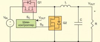
Design and principle of operation

Let's look at the block diagram and algorithm of operation of an analog oscilloscope. As already mentioned, you can change images horizontally and vertically. Devices based on a cathode ray tube (CRT) have two pairs of plates for this purpose. One pair for changing the vertical scale (amplitude or voltage). The second is for horizontal stretching or compression (time parameters).

Analog oscilloscope device: block diagram

The monitored signal is fed to an input amplifier, where it is amplified or reduced to specified values. The value is set by switches. The gain is usually from 100 to 1000. The amplified signal goes to the vertical scanning plates of the cathode ray tube.

The horizontal scan is formed on the basis of a sawtooth signal, which is generated in the corresponding block (scan generator). Its parameters are also set by the corresponding switch. The display on the CRT screen is in real time, with some delay. The delay value is specified in the technical characteristics of the device.

Basic blocks of an analog oscilloscope

The synchronization block is important for the operation of the oscilloscope. It ensures that the picture appears at the moment the potential arrives at the input. Due to this, we see the signal on the screen for a certain period of time. There are different types of synchronization. They are selected by a switch. Most often, synchronization from the signal being studied is chosen. There are also from the network and an external source.

Oscilloscope operating modes

An oscilloscope examines various types of signals. They can be constant (mains voltage), periodic (noise, interference, sounds, etc.). Periodic ones can occur randomly or at regular intervals. Depending on how often or rarely the signal occurs, one or another operating mode is selected. Most often, an oscilloscope has two modes: automatic (self-oscillating) and standby. It could also be one-time.

Selecting the oscilloscope operating mode

If we do not know how often the impulses occur, we usually choose the automatic mode. In it, even if there is no potential at the input or if its level is insufficient, the screen lights up. The “zero” signal is displayed - a straight line that should go along the horizontal axis on the screen (set along the line using the arrow controls). When potential appears at the input, it is displayed on the screen. The picture is periodically updated and we see the signal unfolding over time.

This is what the oscilloscope screen looks like in self-oscillating (auto mode) when there is no signal

Standby mode is good for signals that rarely appear. While there is nothing at the input, the screen does not light up. When any changes occur, it lights up, the sweep generator starts and the signal is displayed on the screen. Triggering can be configured either on the rising edge of the pulse/sine wave or on the descending edge. You can configure the trigger not for the signal being studied, but for the event that precedes it (if there is one).

Single mode configures the oscilloscope to accept a single signal. When the potential of the required level arrives at the input, the signal is displayed on the screen. After this, the device goes into an inactive state. And, even if there is the next potential at the input (or five, or one hundred and five), it will not register it. To receive another pulse, you need to “cock” the device again.

Divider (attenuator)

The signal under study can have a voltage from tenths to hundreds of volts. There are oscilloscopes with a built-in sensitivity control - attenuator. It looks like a graduated switch. It sets the “weight” of one division on the screen and determines how many times the input signal is reduced. If a low level is expected, we simply set it to 1 or 0.1. In this case, one vertical division on the screen will be 1 V and 0.1 V, respectively. And the signal will be “lowered” by 1 time (that is, it will be transmitted as is) or amplified by 10 times before being sent to the input (this is if it is set to 0.1).

Not all oscilloscopes have a built-in divider (attenuator). This device comes with external dividers of 1:10 or 1:100. These are rectangular or cylindrical nozzles with connectors on both sides. They are installed in the input connector and through them the voltage is supplied to the input, but already reduced by the appropriate number of times.

This is what the divider looks like. It is installed in the input socket, and the measuring cord is already connected to it

It is not necessary to set a divisor. The need is determined by the expected signal level. The specifications indicate the maximum input voltage that can be supplied to the device without a divider and with a divider. We set the nozzle according to the level of the expected signal.

If the level is unknown, set the largest divisor first (or the largest division on the attenuator). This will protect the device from burning out if the potential is high. Based on the results of the first measurement, the optimal mode is selected.

Features of digital models

A digital oscilloscope works differently - the analog signal is converted into digital form. In this form, it is recorded in memory and transmitted to the monitor, where it is converted from digital format back into analog form. Display on the screen begins only at the moment when the input level exceeds a certain value (set by settings).

The frequency of changing the picture depends on the selected operating mode: automatic, single and normal. Normal is the equivalent of waiting.

Simplified block diagram of a digital oscilloscope

Why are digital models better? Firstly, this conversion makes the image more stable. Secondly, it's easier to zoom in and out. Thirdly, there is a recording option. Well, and the dimensions. The smallest analog oscilloscope, S1-94, has dimensions of 100*190*300 mm and a weight of 3.5 kg. And digital ones with dimensions of 100*50-60*13-20 mm have a weight of about 150-300 grams. And this includes batteries.

· Part 1 · Part 2 · Part 3 · Part 4 · Part 5 · Part 6 · Part 7 · Part 8 · Part 9 · Part 10 · Part 11 · Part 12 · Oscilloscope.
With and without it · Typical faults. Checks using an oscilloscope · Diagnostics and repair: Do-it-yourself oscilloscope Auto repair. Oscilloscope for troubleshooting, part 7 Continued.
The cause of this malfunction is creeping salts and electrified dust inside the unit. The reference voltage is 5.369V, which is above the permissible deviation.

Photo 10

This signal can be seen at the sensor output when the ignition is on and the engine is not running. The gain value is set by the panel. The signal is quite strong. But neither evil spirits nor other otherworldly forces have anything to do with it. Many, having seen something like this, are lost. A few more oscillograms, and then I will try to explain the essence of what is happening.

Photo 11

Photo 11 shows the sensor signal, which will also mislead the control system. I won’t say what will happen when the signal is digitized. And additional characteristics that give an understanding that the impulse is not ideal are difficult to apply here.

Photo 12.

Photo 12 is also far from bubblegum. The signal must be at a clear frequency. But she's not here. And where does all this come from?

Photo 13

I repeated photo 13 of the rectangular pulse. Now, if you examine it on an oscilloscope as if it were a dark green oscillogram, but at the same time remember that in reality it is like a light green one, then you can find an explanation. To this oscillogram we must also add that most sensors have their own amplifier inside. And the amplifier is not entirely simple. Although from an economic point of view it is cheap, and therefore it is installed in most modern sensors. It is assembled according to a circuit with a common emitter. The amplifier uses negative feedback. Since this is a pulse amplifier, there are some requirements for it. Input signals change quite quickly. And the main indicator for this type of amplifier is the impulse transfer characteristic. Transient processes for such an amplifier are decisive. And for accurate transmission of pulsed signals, phase and dynamic distortions must be kept to a minimum. This is solved by introducing feedback into the amplifier. Part of the signal from the output is fed to the input. The feedback depth is calculated, and any change in it will lead to distortion of the output signal. What can affect it? Yes, the sensor operates in conditions that are not entirely favorable from the point of view of exposure to external factors. One such factor is temperature. And its swings.

Photo14

Here is a sensor that has been in unfavorable conditions (external view)

Photo 15

Photo 16.

Photos 15, 16 are what's inside. The soldering points made with refractory solder have acquired a “coarse” structure and we can talk about contact at the soldering points very conditionally. Even if it exists, the resistance at the solder points has clearly changed no less. This means that it is possible to change the value of the reference voltage inside the sensor itself, and the depth of feedback. That’s why we see “I don’t understand what” at the output. The speed of processes has changed. Phase distortions have emerged. In general, it is advisable to understand this... It seems to me that there is no particular point in analyzing the situation down to formulas for each case, modeling and determining what was the decisive factor: nutrition or changing the depth of feedback. It would be better to replace the sensor. But still, I’ll try to explain why the inversion occurs.

In photo 13, the oscillogram shows a short-term spike in amplitude when it reaches its maximum value. It is short-term and for rectangular pulses it must have a certain time and be a certain part of the maximum value. So, if “something” happens in the amplifier that will allow the process time to be delayed when the maximum surge occurs, and then the time for establishing the maximum amplitude follows (this is a section with damped amplitude oscillations at the maximum) and this time will be equal to the duration of the pulse itself - we will get at the output amplitude significantly exceeding the value of the reference voltage.

We look at the oscillograms, photo 1

And such a signal, with all its beauty and synchronicity, will not work. If this “something” occurs at the moment when the pulse amplitude is in the region of the minimum value emission and the time of establishment of the minimum amplitude, we get a “flip”, oscillogram 2:

That won't work either. It won’t work. If “something” that happened changed the depth of feedback in such a way that it turned the amplifier practically into a generator, leading to self-excitation, then you need to understand that the amplifier still did not lose its input. And since the system contains pulse signals even from the same clock generators, this means that their harmonics are also present. Which, yes, are weak, and even structurally weakened in order to exclude interference on other circuits, but they are there. And they also go to the amplifier input. And who said that they will not play the same role as the modulating signal in the modulator.

The carrier has already appeared, the amplifier is already excited. And then we get this, waveform 3:

For such an oscillogram there may be a question as an application: - “The sensor is in your hand, connected, the ignition is on... what is this?” You can consider more sensors... well, let's look again, but using not an oscilloscope, but a graphical display on a scanner, oscillogram 4:

After analyzing the graphs and data from the scanner and graphs, the decision was made to check the engine in more detail. Why? But because MAF readings directly depend on engine performance. It is not the sensor that “sucks” air, but the engine. And the sensor does not control anything, it simply records how much air has passed through it. And the system specifies - for a “certain period of time” (cycle). The sensor is working, there are no leaks. No, well, you can attack the corrections, the DC, the injectors, the ECU and try to hold them accountable ...

With signals to actuators it is much simpler. There are fewer white spots (which cannot be said about the errors that can be made), oscillogram 5:

There is a fault in the ignition coil.

You can, of course, give oscillograms of injectors, dampers and VVT valves, etc., but it seems to me that enough has already been said to determine the main thing when checking (diagnostics) a car when it does not work or does not work as it should.

What else plays a significant role? Of course, devices. Everyone's equipment is different. Therefore, without focusing on the oscilloscope, we have already given it its importance; we also talked about the scanner... A little can be said about ergonomics and capabilities.

Those who believe that a wide variety of devices allows for a better solution to the problem of troubleshooting... I don’t agree, or I agree, but with a reservation. Sometimes a specialist, using search techniques and completely unremarkable conventional devices, solves the problem no worse than someone who is equipped with dealer equipment. Of course, talking about the capabilities of the first and comparing them with the capabilities of the second is wrong. The capabilities of the devices are different and they not only expand the field of possibilities themselves, but also provide some advantages in the form of special functions. I would like to have a device with advanced capabilities. So that it allows you to reliably determine the malfunction, is easy to use and convenient to use. For example: oscillograms from the secondary ignition system are highly informative and reliable. But using an oscilloscope means... wires, a sensor, it’s a problem to get this sensor where it’s needed... In short, the device cannot be called ergonomic.

But such a device? –(photo by pribor)

It has a flexible probe, you can get it anywhere. Allows you to check any ignition system. Displays the number of revolutions, spark burning time, and breakdown voltage. I took it out, turned it on, brought the probe sensor to the desired point, received data (malfunction on the device screen). Agree, it’s both more convenient and faster than an oscilloscope (But such a device does not exclude an oscilloscope at all, rather it complements it). Various sensors are also not a hindrance, but help in certain moments (discharge, pressure, capacitive, inductive, etc. “stray” sensors... Even homemade ones. But if, using them, you find a malfunction, give up on critics who they puff out their cheeks because they use devices with branded stickers.The result is what is important.

By the way, about sensors, very good data are obtained from the use of an inductive sensor when checking injectors and other actuators. Still, a current oscillogram makes it possible to see a lot. What is not visible when connected directly to the circuit. The tactics for using sensors can be varied and are chosen based on need. A vacuum sensor, for example: it can be used as a probe, but with expanded capabilities, when you need to make sure that the mechanism is working correctly or that the timing belt is installed correctly. In this case, only the sensor signal is taken.

Graphic display of the signal allows you to quickly evaluate the operation of the mechanism.

Photo 18

The signals are simply compared. Visually, But this is already enough. If you need to look at something in more detail, you can do synchronization by injector or coil:

Photo 19.

Here, in photo 19. You can analyze it in more detail and with reference to a specific cylinder. Or, who can forbid you to use a pressure sensor to measure compression and compare it relative to cylinders (skeptics will ask: “why?”... but the compression meter is broken...). Moreover, I know how many Volts on the scale of my oscilloscope will correspond to 1KRA. In other words, no one limits your choice. But with opportunities the situation is somewhat different.

Photo 20

They used to do this too, especially when cars were being prepared for sale. We tightened the XX screw, the damper thrust screw, and turned the distributor body. In other words, “mechanical corrections” were performed, which made it possible to somewhat smooth out the manifestation of the malfunction, which manifested itself in unstable engine operation. Alas, now there is nothing to twist... or so little that the desired result cannot be achieved. The situation can be continued further: the client pays the money and leaves. Then, after some time, he realizes that the problem has not gone away... he goes to another specialist. And that one has more modest opportunities. He may not even be able to see with his instruments what the previous repairman did. And he will scrupulously check and, perhaps, eliminate the malfunction... but he will not get the desired result. And he will return the car, apologizing. Because he couldn’t... And he will be tormented by doubts. And the client will return to the one who had it, the one who made the corrections. And this same specialist, having forgotten what he did last time, simply sets “zeros”, and lo and behold! The machine is like a bird, and the specialist with puffed out cheeks and proudly raised head: “ We are here for you for a reason, we work at the program level

"It's a shame. Yes. But this option is quite possible.

But in this case, the client was lucky: they saw it, returned it to its place, and fixed the problem.

Photo 21

And two more points:

1 - the presence of various devices is not always beneficial. An example is when I was looking for a fault in a Qashqai. A cylinder-by-cylinder power balance test yielded results. But if you have an endoscope, you need to look inside. Visual perception is a convincing thing! ( and for the sake of a control check... and for the sake of curiosity... whatever, for self-affirmation “I’m right”

). Looked in... what did you get? And nothing but doubt. That’s why I didn’t see anything that would confirm the test result! All. And if doubt creeps in, then it’s time to roll “cotton balls”.

2 - I never give advice when asked what equipment is best to buy (options: this, or maybe this?)

Until he starts working, until he holds simple instruments in his hands, a person will not understand and will still have doubts. And when he starts working, the understanding of WHAT he needs will come to him on its own. And then he will be interested in the difference in characteristics and capabilities, based on working conditions.

That's all. It worked out a lot. Possibly stated “grumpily”. But he did not leave the intended line. And if anyone has found even a grain of useful information for themselves, then they wrote it for a reason.

MARKIN Alexander Vasilievich

Nickname on the Legion-Avtodata forum – A_V_M

Belgorod Tavrovo microdistrict 2, Parkovy lane 29B (4722)300-709

How to use an oscilloscope

Initially, the operating mode of the oscilloscope is set (self-oscillating, standby or single). Then the attenuator mode is selected or the appropriate voltage divider is installed. This applies to analog devices. Digital at the input analyzes the signal and lowers/increases it to the required level. They have an analytical unit at the input, which itself lowers or increases the input signal to the required level.

Connecting an oscilloscope

The oscilloscope comes with a test cord or cords. Their number depends on the number of input channels of a particular model. If there is one channel, then there is one cord. Maybe two, three and up to sixteen. You need to connect as much as you intend to use.

Oscilloscope cords are difficult to confuse with others. One end has a probe and a branch. This is the "measuring" side. On the other there is a characteristic round connector. This part is connected to the measuring input.

The wire that goes away from the probe is for connecting to ground. It is often equipped with a clothespin or crocodile clip. It is necessary to connect it, the voltage may be different and grounding is necessary.

Oscilloscope Test Cords

Some oscilloscope cords have a switch on the handle that acts as a small amplifier (pictured at right).

After connecting the measuring cords, turn on the device to the network. Then, before work, we move the toggle switch/button to turn on the device to the working position. We can assume that the oscilloscope is ready for use.

Checking the oscilloscope before use

Before starting work, you need to check the oscilloscope. We plug it into the network and install the measuring cord. We touch the probe with our finger, a sinusoid with a frequency of 50 Hz appears on the screen - interference from the household electrical network.

If you touch the test probe with your finger, a sinusoidal signal will appear on the screen. The sine wave is not ideal, but if it exists and its frequency is 50 Hz, this means that the oscilloscope is working

Then we take the earth probe and touch it to the measuring probe (we continue to keep our finger on the tip of the probe). The signal disappears (a straight line is displayed). This means that the device is working properly.

How to measure voltage with an oscilloscope: alternating, meander, direct

As already mentioned, the voltage on the oscilloscope screen is displayed vertically. The entire screen is divided into squares. The vertical division value is set by a switch labeled “V/div”. Which is what Volts means by one division. Before sending a signal, set the beam exactly along the horizontal axis - this is important.

We give a signal and count how many cells the signal rises or falls from the zero level. Then we multiply the number of cells by the “division price” taken from the regulator. As a result, we obtain the signal voltage. In the case of a sinusoid or meander (positive and negative rectangular pulses), the voltage of the half-wave is considered - upper or lower.

Measuring voltage with an oscilloscope

To make it clearer, let's look at an example. In the photo there is a signal, the half-wave of which is understood and lowered by three cells. The division price on the regulator is 5 V. We have: 3 divisions * 5 V/division = 15 V. It turns out that this signal has a voltage of 15 volts.

If you need to measure DC voltage, again set the beam horizontally. Apply voltage and see how many cells the beam “jumped” or fell. Then everything is exactly the same: multiply by the division price and get the constant voltage value.

How to determine frequency with an oscilloscope

Frequency is defined as 1/T, where T is the period of the signal. And the period is the time during which the signal goes through a full cycle. For a signal on the screen, this is 5.7 cells. We count from the intersection with the horizontal axis to the second similar point.

How to determine the frequency of a signal using an oscilloscope

Next, we determine the division frequency using the sweep switch. The switch position is set to 50 milliseconds. Take the number of divisions and multiply by the number of cells. We get 50 ms * 5.7 = 285 ms. Convert to seconds. To do this, divide by 1000. We get 0.285 seconds. We count the frequency: 1/0.285 = 3.5 Hz

Characterograph for transistors

Using the previous set-top box, you can only check the performance of the transistors. But sometimes such information is not enough to decide on the use of a particular transistor in the device being designed.

var begun_auto_pad = ; var begun_block_id = ;

After all, it is often necessary to select transistors, say, for the output stage of a radio receiver, with the same or possibly similar parameters. The most acceptable practical way here is to measure the static current transfer coefficient. But the best results are obtained by comparing the output characteristics of transistors and selecting devices with the same data based on them.

The story will be about an attachment to an oscilloscope for viewing the output characteristics of transistors of both structures - a curve tracer. But before we start, we should say a few words about the output characteristics and answer the question of why they were chosen for control by a characterograph.

The output characteristics of the transistor are the dependences of the collector current on the voltage between the collector and the emitter at various base currents. Such characteristics are usually taken when the transistor is switched on according to a common emitter (CE) circuit. Here, for example, is how this is done for the MP42B transistor (Fig. 13, a). Using a variable resistor RI connected to the galvanic element G1, the base current of the transistor is changed, and the voltage at the collector is set with a variable resistor R2 connected to the battery GB1 (for example, composed of eight elements (voltage 1.5 V). The base current is controlled with a microammeter PA1 , collector - with milliammeter RA2, and the voltage between the collector and emitter - with voltmeter PV1.

Having set the base current, say, equal to 20 μA, a voltage of 1 V, 2 V, 3 V, etc. is applied to the collector. For each voltage value, the value of the collector current of the transistor is determined. Then other values of the base current are set (40, 60, 80 μA, etc. and the collector current is again determined at different voltages on the collector. And then, using the data obtained, a graph is drawn (Fig. 13.6) of the family of output characteristics of this transistor. Similar you will find graphs in reference books on transistors.What do the output characteristics indicate?Firstly, the output current, i.e., the collector current, almost does not depend on the voltage on the collector, but is determined only by a given base current.

Secondly, “with an existing cascade power source, the specified collector current can be provided at a very specific base current. Let's say that if you need a collector current of 4.5 mA at a power supply voltage of 4.5 V, the base current should be 40 μA. And for a collector current of 8 mA with the same power supply, you will have to increase the base current to 80 μA. This is how you can determine the desired “initial base current” from the output characteristics, and then use it to calculate the resistance of the base resistor.

In addition, from the output characteristics it is not difficult to determine the output resistance of the transistor for direct or alternating current - parameters that need to be known to calculate the amplifier stages and properly match them. For example, the DC resistance at operating point A will be;

R_ =Uk /Ik where R_ is the transistor resistance, Ohm; UK is the voltage at the transistor collector, V; Ik is the collector current, A. In our example, the resistance will be 1000 Ohms. At point B the resistance will be lower.

For alternating current, the resistance at the same point A can be determined by the formula:

R ~=ΔUK /ΔIK , where R~ is the transistor resistance, kOhm; ΔUK—voltage increment at the collector, V; ΔIк is the corresponding increment in the collector current, mA. For those shown in the graph in Fig. 13b increments, it is easy to calculate that the transistor resistance will be approximately 15 kOhm.

And further. Based on the output characteristics, it is possible to determine the static transfer coefficient of the base current at a given operating point. To do this, you need to divide the value of the collector current by the base current. Let's say, for point A the transmission coefficient will be 105, at point B it will decrease to 100. Do you see how much useful information was obtained from the output characteristics of the transistor? That is why, by comparing different output characteristics with each other, it is possible to more accurately select transistors with identical parameters.

And now about our attachment device. Its task is to supply the transistor under test with a varying collector voltage and a stepwise changing base voltage, which determines the base current. The current “steps” must be the same. Then on the screen of an oscilloscope connected to the collector circuit of the transistor, it will be possible to “see” the output characteristics.

The diagram of a practical attachment-character, developed by Kursk radio amateur Igor Aleksandrovich Nechaev, is shown in Fig. 14. The set-top box is powered by an alternating current network, the voltage of which is supplied by switch Q1 to step-down transformer T1. From the secondary winding, voltage is supplied to two rectifiers. The first is made using diode VD1, smoothing filter C1R1C2 and zener diode VD3. It is used to power the set-top box chips.

The second rectifier, on diode VD2, provides the pulsating voltage necessary to power the collector circuit of the transistor being tested and obtain a horizontal scan line of the oscilloscope.

A generator of rectangular pulses is assembled on elements DD1.1 and DD1.2, traveling at a relatively high frequency - about 100 kHz. They go to the inverter DD1.3 and the frequency divider by 2, made on the trigger DD2. A so-called digital-to-analog converter made up of resistors R5-R8 is connected to the outputs of the inverter and trigger. At point A of the converter, a step voltage is generated, shown in Fig. 15, a.

When the tested transistor of the np-p structure is connected to the sockets “E”, “B”, “K” of the XS1 connector, and the switches SB1 and SB2 are set to the position shown in the diagram, a pulsating voltage is supplied to the transistor collector, varying in amplitude from zero to 20 V. At the same time, a step voltage is supplied to the base of the transistor from the digital-to-analogue converter, but through a chain of series-connected resistors R9 and R10. With the variable resistor R10 you can change this voltage, and therefore the current in the base circuit. Moreover, when the resistor slider is moved, the base current from each voltage “step” changes proportionally.

The current flowing in this case (it is also “stepped”) through the transistor creates a “stepped” voltage drop across resistor R11, connected to the emitter circuit of the transistor. The voltage taken from the resistor is supplied through the HRZ plug to the vertical input of the oscilloscope. The “ground” probe of the oscilloscope is connected to the XP4 plug, and the signal from the XP2 plug is fed to the horizontal input of the oscilloscope. Since the frequency of changes in the “steps” of the current at the base of the transistor is significantly 2000 times higher than the sweep frequency, almost continuous (although in fact they are from separate points) images of the output characteristics of the transistor appear on the screen (Fig. 15, b).

It should be immediately clarified that in this case it is not the collector, but the emitter current that is observed, which practically coincides with the collector (the difference can be tens of microamperes, which is not significant for our measurements). The XS2 connector sockets are used to connect a second transistor of a similar structure to the console. By pressing and releasing the SB1 button, you can observe the output characteristics of either the first or second transistor on the oscilloscope screen and compare them with each other.

When you need to check transistors of the pnp structure and compare them with each other, use connector sockets XS3 and XS4. But in this case, the step voltage and the base of the transistor are supplied through the so-called “current mirror”, composed of transistors VT1 and VT2. It ensures the same polarity of the signal based on the transistor of the pnp structure in relation to the emitter as in the case of checking a transistor of a different structure. As a result, the picture of the output characteristics on the screen remains unchanged when testing transistors of any structure.

The curve graph attachment allows you to observe on the screen the output characteristics for four values of the base current (one of the currents is zero). Of course, a greater number of gradations of the base current is possible, but, unfortunately, on the small-sized OML-2M (OML-ZM) screen they will be poorly distinguishable. Moreover, the design of the console will become more complicated.

In addition to those indicated in the diagram, the set-top box can use microcircuits K176LE5, K561LE5, K561LA7 (DD1), K561TM2 (DD2); transistors KT315A—KT315I with possibly similar parameters; diodes KDYu2B, KDYUZA, KDYu5B—KDYu5G, D226B; Zener diode D809. Fixed resistors can be of types MLT, BC, variable R10—SPO-0.5, OLZ-12. Capacitors C1, C2 - K50-3, K50-6, K50-12; SZ - MBM, BM, KLS; C4 - CD, CT, CLS. Switch Q1—P2K with position fixation, switch SB2—also P2K with position fixation, and SB1—similar, but without position fixation. Sockets from K155 series microcircuits were used as connectors for connecting transistor outputs, but other small-sized connectors with sockets are also suitable.

Power transformer T1 is ready-made, from the Alpinist-417 radio receiver. You can use any other low-power and small-sized transformer with a voltage on the secondary winding of 12V at a load current of up to 100 mA. Some parts of the set-top box are mounted on a printed circuit board (Fig. 16), and some are installed on the front panel - the cover of the metal case (Fig. 17). The board is mounted on the side wall of the case.

You will check and adjust the set-top box using an oscilloscope operating in automatic mode, with an open input and a sensitivity set to 10 V/div. First, connect the input probes of the oscilloscope to the terminals of the secondary winding of the transformer and check the range of the alternating voltage - the swing of oscillations here will be about 40 V (Fig. 18, a). Then connect the oscilloscope's ground probe to the XP4 plug, and the input probe to the XP2 plug. Now half-wave oscillations with an amplitude of about 20 V will appear on the screen (Fig. 18.6).

Next, connect the input probe to the positive terminal of capacitor C1—you will see a winding line approximately two divisions away from the scan line (Fig. 18, c). This is rectified voltage with ripples. The level of ripple can be easily measured by switching the oscilloscope to the closed input mode and setting the sensitivity to 1 V/div - it will be almost 3 V.

Having moved the input probe of the oscilloscope (it again operates in open input mode) to the output of the zener diode cathode, you will see an almost straight line (Fig. 18d), raised above the scan line by almost a division. This is the supply voltage of the microcircuits, stabilized by a zener diode. Its ripple level does not exceed 0.05 V, which is quite acceptable for our purposes.

Let's move on to checking the generator part of the set-top box. It is also convenient to use the oscilloscope in open input mode here. The scan is still in automatic mode with internal synchronization. Using the input probe of the oscilloscope, touch pin 10 of element DD1.3. Two parallel lines will appear on the screen. You need to select a sweep duration, for example, equal to 5 μs/div., and then turn on the standby mode on the oscilloscope with triggering from a positive signal. Generator pulses will appear on the screen (Fig. 19, a). The tops of the pulses are the levels of logical 1, and the areas at the base are the levels of logical 0. The leading edges of the pulses are 10 µV apart, which means their repetition frequency is 100 kHz.

Transfer the input probe of the oscilloscope to pin 1 of the DD2 trigger - here the pulses are wider (Fig. 19.6) and follow at half the frequency.

The result of the summation of both signals (from the outputs of element DD1.3 and the trigger), in other words, the result of the operation of the analog-to-digital converter, will be seen at point A connections of the terminals of resistors R6, R8, R9 (Fig. 19, c). To get a better view of the image, increase the oscilloscope sensitivity to 2 V/div. and shift the scan line, for example, to the lower division of the scale grid (Fig. 19,d).

Isn't it true that there is a stepwise increase in the signal? But the “steps” look smoothed out, barely similar to those shown in Fig. 15, a. The oscilloscope is at fault. After all, its input capacitance is relatively large (40 pF), and the observation of a very short (5 microns in duration for each “step”) pulse signal is carried out in a divider with a relatively high resistance of resistors. The signal is integrated, and the leading edges of the pulses “fall over”.

How to get rid of this “defect”? It is necessary to reduce the input capacitance of the measuring circuit by connecting the input probe of the oscilloscope to the specified point through a small capacitor - 10 ... 5 pF. You will see clear “steps” on the screen, however, to observe them you will have to increase the sensitivity of the oscilloscope. And so that the image is not distorted by the findings, you will have to either solder the probe (the conductor from it) to the point being checked, or touch the “ground” probe with your other hand if you hold the input one in your hand.

After this, you can connect the input probe of the oscilloscope to the XP3 plug (or insert the plug directly into the input socket of the oscilloscope), and connect the XP2 plug to the “In” socket. X (SYNC.)" oscilloscope through a variable resistor with a resistance of 100 kOhm. The oscilloscope should now operate in external sweep mode (the “SEL—INX” button is pressed) with an open (or closed) input. Using an additional variable resistor, set the length of the scan line to eight divisions, and shift the line itself to the lower division of the scale grid (Fig. 20, a). Since the amplitude of the voltage coming from the XP2 plug is 20 V, the line division price will correspond to 2.5 V.

Set the console switches to the position shown in the diagram, and the variable resistor R10 slider to approximately the middle position. Insert a transistor, say, KT315B, into the sockets of the XS1 connector. A picture of the output characteristics should appear on the oscilloscope screen, which can be set convenient for observation (Fig. 20.6) by changing the sensitivity of the oscilloscope (for example, by setting the sensitivity to 0.2 V/div). When you move the slider of the variable resistor R10, the distance between the branches of the characteristics will change - the image will either be compressed or stretched. But it is impossible to say anything specific about the parameters of the transistor, for example about its transmission coefficient, since the scale of the variable resistor and the value of the base current, as well as its increments, have not yet been calibrated.

Let's start calibrating the scale of the variable resistor. Temporarily disconnect resistor R3 from the common passage and connect the freed pin to socket “B” of connector XS3. In parallel with resistor R3, connect the input probes of the oscilloscope (the “ground” probe - to the top terminal of the resistor in the diagram), operating in automatic mode, with internal sweep. Set the sweep duration to 5 µV/div, and the sensitivity to 0.05 V/div.

Switch SB2 to the “p-p-p” position and turn on the console. A signal will appear on the oscilloscope screen, the range of which depends on the sensitivity. If it is sufficient (3 divisions), you can switch the oscilloscope to standby mode and synchronize the image. These will be mirrored (compared to those shown on cassocks, 15 and 19) “steps” (Fig. 20, d).

By moving the variable resistor R10, you can change the amplitude of the “steps”, i.e., change the current flowing through resistor R3, and therefore through the future base circuit of the transistors being tested.

Having set the resistor slider to the position of maximum resistance (i.e., minimum base current), measure the amplitude of any of the “steps” (they should be the same), and then calculate the increment of the base current using the formula:

Δ /6=106-Uc /R 3, where ΔIb is the increment of the base current, μA; Uc is the “step” amplitude, V; R3 - resistance of resistor R3, Ohm. The resulting value is indicated on the resistor scale.

Similarly, the values of current increments in intermediate and other extreme positions of the resistor slide are determined and marked on the scale. In general, it is enough to put 4-5 values on the scale, say, 30, 40, 50, 75, 100 µA. Now you can restore the connection of resistor R3 to the common wire and return to observing the output characteristics. And from them, determine the transmission coefficient (Fig. 20, c) using the formula:

h 21e=106ΔU /Δ /I b*R 11, where h21e is the transmission coefficient of the transistor; ΔU—step amplitude, V; ΔIb—base current increment value set by variable resistor R10, μA; R11—resistance of resistor R11, Ohm.

In the one shown in Fig. 20, in the example, the variable resistor R10 slider was in the “50 μA” position, and the sensitivity of the oscilloscope was set to 0.2 V/div. Therefore, the transmission coefficient of the transistor was 80. When connecting other transistors, try to determine their transmission coefficient. By inserting a pair of np-n structure transistors into sockets XS1 and XS2, and a pair of pnp structure transistors into sockets XS3 and XS4, you can compare them with each other with a friend based on observable characteristics.

When working with the set-top box, remember that it is designed for testing low-power transistors. In addition, the high frequency of changes in the “steps” of the base current makes it difficult to test low-frequency transistors (for example, MP26B). If you still want to use the attachment for such transistors, it is recommended to change (reduce) the frequency of the generator by increasing the resistance of resistor R4 up to 3 MOhm.

It may happen that with transistors VT1 and VT2 installed, the “current mirror” will not work reliably. Then you will have to slightly change its circuit - insert resistors with a resistance of 20 kOhm into the emitter circuits of the transistors, and move resistor R9 into the circuit of the upper, according to the diagram, contact of section SB2.1 of the structure switch.

On the charachteriograph set-top box, you can check, as on the previous set-top box, semiconductor diodes and zener diodes - their terminals are connected to the “K” and “E” sockets of connectors XS1 and XS2.

And one last thing. The curve-character attachment is suitable, in addition to the OML-2M (OML-ZM), for other oscilloscopes equipped with an external scan socket (horizontal deflection amplifier input). Depending on the sensitivity of this input, the resistance of the external additional resistor in the XP2 plug circuit is selected to obtain the desired scan line length.

If this character graph makes it possible to observe four dependences of the collector current on the collector-emitter voltage at fixed base currents, then with the help of attachments developed by the Bryansk radio amateur V. Inozemtsev, eight such characteristics appear on the oscilloscope screen.

Figure 21 shows a diagram of the first version of the curve-character attachment, designed to test low-power transistors of both structures. Moreover, the leads of transistors of the np-p structure are connected to sockets XS1-XS3, and the leads of transistors of the p-n-p structure are connected to sockets XS4-XS6.

Fixed base currents of the transistors under study are obtained due to the inclusion in the base circuit of “weighting” (i.e., multiples of some value - “weight”) resistors R13 (R), R12 (2R), Rll (4R) using electronic switches VT5, VT4 and VT3 respectively. In turn, the electronic keys are controlled by signals from the outputs of the counter DD1, therefore, depending on the states of the counter, eight base current values are obtained: 0, 1b, 21b, ... 71b.

The counter is switched by pulses with a frequency of 100 Hz—they are supplied to input C2 of the counter from the collector of transistor VT2. The signal to the base of this transistor in the form of a pulsating voltage with a frequency of 100 Hz is supplied from the VD5 diode.

A rectifier is assembled using diodes VD1-VD5 to power the base circuit of the transistor under study and the DDL microcircuit. The voltage to the microcircuit is supplied from a parametric stabilizer made on resistor R1 and zener diode VD7 and connected to the rectifier. Another parametric stabilizer, made on resistor R2 and zener diode VD6, is used to obtain the voltage that supplies the base circuit of the transistor being tested, in other words, the voltage that determines the currents through resistors R11-R13. So that these currents can be changed depending on the transmission coefficient of the transistor under study, a regulating transistor VT1 is introduced into the stabilizer, to the base of which the voltage from the parametric stabilizer is supplied through a variable resistor R3. When the position of the slider of this resistor changes, the voltage on the load resistor R5 changes, which means that the “portions” of current in the base circuit of the transistor under study change when the keys on transistors VT3-VT5 are opened. To limit the current, resistors R8-R10 are installed in the basic circuits of the key transistors.

Another rectifier is assembled using diodes VD8-VD11, but without a filter capacitor at the output. Therefore, a pulsating voltage with a frequency of 100 Hz is removed from it, which is used to power the collector-emitter circuit of the transistor under study. The voltage from resistor R14, proportional to the collector current of the pn-p structure transistor or the emitter current of the pn-p structure transistor, is supplied to the vertical input of the oscilloscope. Since in the connection circuit of the OE transistor (common emitter) the collector current differs slightly from the emitter current, it turned out to be possible to include resistor R14 in the emitter circuit of the studied transistor of the p-p-p structure. With this construction of the measuring circuit, the oscilloscope beam shifts from the zero position to the right and upward, i.e., the characteristics are convenient for observation.

The direction of the current in the base circuit, depending on the structure of the transistor under study, is changed by switch SA1.

Alternating voltages can only be supplied to the rectifiers from different windings of the transformer. Moreover, the winding from which the voltage is removed to the diodes VD1-VD4 must have the smallest possible capacitive coupling with the mains winding, otherwise voltages may appear in the image at the mains frequency. The easiest way to reduce this connection is to use a U-shaped magnetic core for the transformer and place the windings on different magnetic cores. Interference at higher frequencies that can penetrate from the network is filtered by capacitor C2.

Most of the parts indicated in the diagram can be mounted on a printed circuit board (Fig. 22) made of fiberglass 1.5 mm thick. Since the oxide capacitor C1 uses a relatively large capacitance, it can be composed of several capacitors of smaller capacitance (for example, 1000 μF) connected in parallel. For this purpose, the board provides space and additional holes for K50-6 capacitors.

If you intend to test only transistors of the np-p structure, you can assemble a simpler attachment-characterizer according to the circuit shown in Fig. 23. In this case, no special requirements are imposed on the transformer from which the 10 V alternating voltage is removed.

“Weighting” resistors (R11-R13 in Fig. 21 and R4-R6 in Fig. 23) are selected depending on the required base currents. To study low-power transistors, a “weight” of 20 kOhm was selected. When studying more powerful transistors, it may be different. But in any case, the ratio of the resistances of resistors R13, R12 and Rll (R6, R5 and R4 for Fig. 23) should remain equal to 1: 2: 4.

. Oscilloscope attachments

Oscilloscope bandwidth: what it is and what it affects

When choosing an oscilloscope, look at the following parameters:

Bandwidth.
Maximum input voltage.
Sweep modes.
Synchronization sources.

All parameters except bandwidth have already been discussed. Bandwidth is almost the most important indicator. It determines the maximum signal frequency that will be displayed without distortion. For example, with a bandwidth of 20 Hz - 20 MHz, anything with a higher frequency will be suppressed.

Where bandwidth ends, frequencies are severely suppressed

How to choose the transmission frequency? Depends on what signals you are going to study and how “deep” you need to study them. For analog signals everything is simple - the upper limit must be greater than the maximum frequency. With meanders everything is more complicated. In fact, they consist of the sum of the odd harmonics of the signal. The more harmonics, the more the shape looks like a square rather than something smoothed out. But high order harmonics have a very high frequency. If you need to study the fronts and their deflection, then the upper limit of the bandwidth is tens of gigahertz. And such devices are very expensive. For a regular sine wave, 10-20 MHz is enough, which is much cheaper.