In practice, there are often problems of calculating the parameters of currents and voltages in various branched circuits. Kirchhoff's rules are used as a tool for calculations (in some literature they are also called laws, although this is not entirely correct) - one of the fundamental rules that, together with Ohm's laws, allows one to determine the parameters of independent circuits in the most complex circuits.
The scientist Gustav Kirghoff formulated two rules [], for the understanding of which the concept of a node, branch, and contour was introduced. In our situation, we will call a branch a section through which the same current flows. The connecting points of the branches form nodes. The branches, together with the nodes, form contours - closed paths along which current flows.
Story
Kirchhoff joined the ranks of German scientists in the nineteenth century, when the country, which was on the threshold of the industrial revolution, required the latest technology. Scientists were searching for solutions that could accelerate industrial development.
They were actively involved in research in the field of electricity, because they understood that it would be widely used in the future. The problem at that time was not how to make electrical circuits from possible elements, but how to carry out mathematical calculations. This is where the laws formulated by the physicist appeared. They were very helpful.
The algebraic sum of currents arriving at a node and leaving it is equal to zero. This simultaneously follows from another law - the constancy of energy.
2 wires go to the node, and one goes out. The value of the current flowing from the node is the same as the sum of it flowing through the other two conductors, i.e. going to him. Kirchhoff's rule explains that, in a different situation, a charge would accumulate, but this does not happen. Everyone knows that any complex chain can be easily divided into separate sections.
But it is not easy to determine the path along which it passes. Moreover, in different areas the resistance is not the same, therefore the distribution of energy will not be uniform.
In accordance with Kirchhoff's Second Rule, the energy of electrons in each of the closed sections of the electrical circuit is equal to zero - the total value of voltages in such a circuit is always equal to zero. If this rule were violated, the energy of electrons passing through certain areas would decrease or increase. But this is not observed.
Loop current method
When calculating complex circuits, the loop current method is used. This method is a consequence of Kirchhoff's rules . A complex contour is considered as a collection of simple closed contours. This method assumes that the same current flows in all sections of each closed loop. These currents are called busturns. The total current strength that flows through a section of the circuit is equal to the algebraic sum of the strengths of the circuit currents for which this section is common. Kirchhoff's equation is written in terms of loop currents. In this case, the number of equations for loop currents is equal to the number of unknown currents.
Conductor connections
There are two main ways to connect conductors to each other - series and parallel connections. Various combinations of series and parallel connections result in a mixed connection of conductors.
Resistors and lead wires
We call a conductor with a resistance R a resistor and depict it as follows (Fig. 1):
Rice. 1 Resistor
The voltage across a resistor is the potential difference in a stationary electric field between the ends of the resistor. Between which ends exactly? In general, this is not important, but it is usually convenient to match the potential difference with the direction of the current.
The current in the circuit flows from the “plus” of the source to the “minus”. In this direction, the potential of the stationary field decreases. Let us remind you again why this is so.
Let a positive charge q move along the circuit from point a to point b, passing through resistor R (Fig. 2):
Fig.2 U = φa – φb
In this case, the stationary field does positive work A = q(φa − φb). Since q > 0 and A > 0, then φa − φb > 0, i.e., φa > φb.
Therefore, we calculate the voltage across the resistor as the potential difference in the direction of the current: U = φa − φb.
The resistance of the lead wires is usually negligible; on electrical diagrams it is considered equal to zero. It then follows from Ohm’s law that the potential does not change along the wire: after all, if φa − φb = IR and R = 0, then φa = φb (Fig. 3):
Fig.3 φa = φb
Thus, when considering electrical circuits, we use an idealization that greatly simplifies their study. Namely, we believe that the potential of a stationary field changes only when passing through individual elements of the circuit, and remains unchanged along each connecting wire. In real circuits, the potential decreases monotonically when moving from the positive terminal of the source to the negative.
Serial connection
When connecting conductors in series, the end of each conductor is connected to the beginning of the next conductor.
Consider two resistors R1 and R2 connected in series and connected to a constant voltage source U (Fig. 4). Recall that the positive terminal of the source is indicated by a longer line, so the current in this circuit flows clockwise.
Let us formulate the basic properties of a serial connection and illustrate them with this simple example:
- When the conductors are connected in series, the current strength in them is the same. In fact, the same charge will pass through any cross section of any conductor in one second. After all, charges do not accumulate anywhere, they do not leave the circuit outside and do not enter the circuit from the outside.
- The voltage in a section consisting of series-connected conductors is equal to the sum of the voltages on each conductor. Indeed, the voltage Uab in section ab is the work of the field to transfer a unit charge from point a to point b; voltage Ubc in section bc is the work done by the field to transfer a unit charge from point b to point c. Added up, these two works will give the work of the field to transfer a unit charge from point a to point c, that is, the voltage U over the entire section: U = Uab + Ubc.
We recommend reading: Electricity - what is it, where does it come from, in what year was it invented
? You can do it more formally, without any verbal explanation: U = Uac = φa − φc = (φa − φb) + (φb − φc) = Uab + Ubc.
- The resistance of a section consisting of series-connected conductors is equal to the sum of the resistances of each conductor. Let R be the resistance of section ac. According to Ohm's law we have:
which is what was required.
You can give an intuitive explanation of the rule for adding resistances using one particular example. Let two conductors of the same substance and with the same cross-sectional area S, but with different lengths l1 and l2, be connected in series.
The resistances of the conductors are equal:
But this, we repeat, is only a particular example. The resistances will also add up in the most general case - if the materials of the conductors and their cross sections are also different. The proof of this is given using Ohm's law as shown above. Our proofs of the properties of a series connection, given for two conductors, can be transferred without significant changes to the case of an arbitrary number of conductors.
Parallel connection
When connecting conductors in parallel, their beginnings are connected to one point in the circuit, and their ends are connected to another point.
Again we consider two resistors, this time connected in parallel (Fig. 5).
Resistors are connected to two points: a and b. These points are called nodes or branch points of the chain. Parallel sections are also called branches; the section from b to a (in the direction of current) is called the unbranched part of the circuit.
Now let’s formulate the properties of a parallel connection and prove them for the case of two resistors shown above:
- The voltage on each branch is the same and equal to the voltage on the unbranched part of the circuit. In fact, both voltages U1 and U2 across resistors R1 and R2 are equal to the potential difference between the connection points:
U1 = U2 = φa − φb = U.
This fact serves as the most clear manifestation of the potentiality of a stationary electric field of moving charges.
- The current strength in the unbranched part of the circuit is equal to the sum of the current strengths in each branch. Let, for example, let a charge q arrive at point a during time t from an unbranched section. During the same time t, charge q1 leaves point a to resistor R1, and charge q2 goes to resistor R2. It is clear that q = q1 + q2. Otherwise, a charge would accumulate at point a, changing the potential of this point, which is impossible (after all, the current is constant, the field of moving charges is stationary, and the potential of each point in the circuit does not change with time). Then we have:
which is what was required.
- The reciprocal value of the resistance of a section of a parallel connection is equal to the sum of the reciprocal values of the resistances of the branches. Let R be the resistance of the branched section ab. The voltage in section ab is equal to U; the current flowing through this section is equal to I. Therefore:
Reducing by U, we get:
1/R = 1/R1 + 1/R2 ,
which is what was required.
As in the case of a series connection, this rule can be explained using a particular example without resorting to Ohm's law.
Let conductors from the same substance with the same lengths l, but different cross sections S1 and S2, be connected in parallel. Then this connection can be considered as a conductor of the same length l, but with a cross-sectional area S = S1 + S2. We have:
The above proofs of the properties of a parallel connection can be transferred without significant changes to the case of any number of conductors.
From relation (1) you can find R:
R = R1R2/(R1 + R2) .
Unfortunately, in the general case of n parallel-connected conductors, a compact analogue of formula (2) does not work, and one has to be content with the relation
1/R = 1/R1 + 1/R2 + . . . + 1/Rn.
Nevertheless, one useful conclusion can be drawn from formula (3). Namely, let the resistances of all n resistors be the same and equal to R1. Then:
We see that the resistance of a section of n identical conductors connected in parallel is n times less than the resistance of one conductor.
Mixed compound
A mixed connection of conductors, as the name suggests, can be a set of any combinations of series and parallel connections, and these connections can include both individual resistors and more complex composite sections.
The calculation of a mixed connection is based on the already known properties of serial and parallel connections. There is nothing new here: you just need to carefully divide this circuit into simpler sections connected in series or in parallel.
Let's consider an example of a mixed connection of conductors (Fig. 6).
Rice. 6 Mixed connection
Let U = 14 V, R1 = 2 Ohm, R2 = 3 Ohm, R3 = 3 Ohm, R4 = 5 Ohm, R5 = 2 Ohm. Let's find the current strength in the circuit and in each of the resistors.
Our circuit consists of two sections connected in series ab and bc. Section resistance ab:
We recommend reading: Switching power supply: what is it, principle of operation, circuit, purpose
Circuit resistance: R = Rab + Rbc = 1.2 + 1.6 = 2.8 Ohm.
Now we find the current strength in the circuit:
I = U/R = 14/2.8 = 5 A.
To find the current in each resistor, let's calculate the voltage in both sections:
Uab = IRab = 5 1.2 = 6 V;
Ubc = IRbc = 5 1.6 = 8 V.
(Note in passing that the sum of these voltages is equal to 14 V, i.e., the voltage in the circuit, as it should be with a series connection.)
Both resistors R1 and R2 are at voltage Uab, therefore:
Therefore, current flows through resistor R5 I5 = I − I3 = 5 − 1 = 4 A
Kirchhoff's laws
Kirchhoff's laws are rules that show how currents and voltages relate in electrical circuits. These rules were formulated by Gustav Kirchhoff in 1845. In the literature they are often called Kirchhoff's laws, but this is not true, since they are not laws of nature, but were derived from Maxwell's third equation with a constant magnetic field. But still, the first name is more familiar to them, so we will call them, as is customary in the literature, Kirchhoff’s laws.
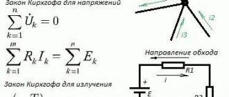
Kirchhoff's first law
Kirchhoff's first law says that the sum of the currents in any node of an electrical circuit is zero. There is another formulation that is similar in meaning: the sum of the values of the currents entering the node is equal to the sum of the values of the currents leaving the node.
Let's look at what has been said in more detail. A node is a junction of three or more conductors.
The current flowing into a node is indicated by an arrow pointing towards the node, and the current leaving the node is indicated by an arrow pointing away from the node. According to Kirchhoff's first law, we conventionally assigned the sign “+” to all incoming currents, and “-” to all outgoing currents. Although this is not important.
Kirchhoff's 1st law is consistent with the law of conservation of energy, since electrical charges cannot accumulate in nodes, therefore, charges arriving at a node leave it.
A simple circuit consisting of a power source with a voltage of 3 V (two 1.5 V batteries connected in series), three resistors of different values: 1 kOhm, 2 kOhm, 3.2 kOhm (you can use resistors of any other ratings). We will measure the currents with a multimeter in the places indicated by the ammeter.
If we add up the readings of three ammeters, taking into account the signs, then, according to Kirchhoff’s first law, we should get zero:
I1 – I2 – I3 = 0.
Or the readings of the first ammeter A1 will be equal to the sum of the readings of the second A2 and third A3 ammeters.
Kirchhoff's second law and its definition
In a single closed circuit, the algebraic sum of the EMF will be equal to the value that sums up the voltage changes for the total number of resistive elements of a given circuit.
Kirchhoff's second rule is relevant in networks with direct and/or alternating current. In the formulation of the law, it is the concept of algebraic sum that is used, since it can be indicated with a plus or minus sign. An accurate determination is only possible in this case through a simple but effective algorithm. First, you need to choose some direction to go around the contour, clockwise/counterclockwise, at your own discretion. The direction of the current itself is selected only through the elements of the circuit. Then you should determine the signs “+” and “-” for voltages and EMF. Voltages should be written with a negative sign when the current does not correspond to the circuit bypass in terms of direction and with a plus in case of coincidence. The same rule should be used in the case when it is necessary to note the EMF.
Laws for magnetic field
Kirchhoff's rules have also found their application in the calculation of magnetic circuits. Kirchhoff's first law for a magnetic circuit looks like this:
Simply put, the sum of all magnetic fluxes passing through a node is zero.
The second law, as applied to magnetic fields, is as follows: “The sum of the magnetomotive forces in a circuit is equal to the sum of the magnetic stresses.” The formula looks like this:
Kirchhoff derived rules that have an absolute applied nature. With their help you can solve practical problems in electrical engineering. The widespread use of these rules is explained by the simplicity of the formulation of the equations and the possibility of solving them using standard methods of linear algebra.
The meaning of Kirchhoff's rules
Kirchhoff's laws express the fundamental principles of physics. Their formulations seem very simple and obvious. But in fact, they represent a method that allows you to calculate the electrical parameters of networks of very complex configurations.
Using Kirchhoff's laws, you can create a system of independent equations to calculate the parameters of an electrical circuit. It is important that their number is no less than the number of parameters that need to be determined.
The figure below shows the electrical circuit for which the calculation will be carried out. Using the first law or Kirchhoff's rule, for node A we can write:
I = I1 + I2.
Two currents enter this node and one exits. Next, you need to apply the second rule. To do this, you can select the outer contour. It can be seen that there are two current sources and two resistors. Therefore, the following equations will be obtained:
Here are 2 equivalent formulas. The left side of the equation takes into account the electromotive forces of the two current sources, the right side takes into account the voltage drop across both resistors, taking into account the direction of the currents. Another equation can be obtained from the 2nd law when walking along the right inner contour:
We recommend reading: How field-effect transistors work; a simplified explanation of electronic switch circuits, current regulators, amplifiers in
The result is a system that includes three equations with three unknowns:
Using specific data, you can substitute numerical values into the system of equations and find what the current strength is for each branch belonging to node A. When making calculations, it is important to understand that with a fairly complex electrical circuit configuration, it is sometimes difficult to determine the direction of the current strength for each branch.
The first and second laws of Gustav Kirchhoff make it possible to accurately determine not only the magnitude of the current, but also its sign. If in the given example, after calculating the desired values using the presented system of equations, it turns out that the current with index 2 takes a negative value, then this means that in fact it has the direction opposite to that indicated in the figure.
Calculations of electrical circuits using Kirchhoff's laws
Rotation speed: formula
To perform such calculations of electrical circuits, there is a certain algorithm in which the currents for each branch and the voltage at the terminals of all elements included in the EC are calculated. In order to calculate any scheme, adhere to the following order:
- The EC is divided into branches, contours and nodes.
- Arrows indicate the expected directions of movement of I in the branches. Arbitrarily mark the direction in which the contour is walked around when writing equations.
- Write equations using Kirchhoff's first and second rules. In this case, the rules of signs are taken into account, namely:
- “plus” are currents flowing into the node, “minus” are currents flowing out of the node;
- E (EMF) and the reduction in voltage across resistors (R*I) are denoted by a “plus” sign if the current and bypass are the same in direction, or “minus” if not.
- By solving the resulting equations, the required values of currents and voltage drops across the resistive elements are found.
Information. Independent nodes are those that differ from others in at least one new branch. Branches containing EMF are called active, while branches without EMF are called passive.
As an example, we can consider a circuit with two EMFs and calculate the currents.
Example of a diagram for calculations with two E
The direction of currents and circuit bypass is arbitrarily chosen.
Intended directions on the diagram
The following equations are compiled using Kirchhoff’s first and second laws:
- I1 – I3 – I4 = 0 – for node a;
- I2 + I4 – I5 = 0 – for node b;
- R1*I1 + R3*I3 = E1 – acef circuit;
- R4*I4 – R2*I2 – R3*I3 = – E2 – circuit abc;
- R6*I5 + R5*I5 + R2*I2 = E2 – bdc circuit.
Equations are solved using determinant or substitution methods.
Using Kirchhoff's law on voltages in a complex circuit
Kirchhoff's voltage law can be used to determine an unknown voltage in a complex circuit where all other voltages along a specific "loop" are known. As an example, take the following complex circuit (actually two series circuits connected by a single wire at the bottom):
Figure 10 – Kirchhoff’s voltage rule in a complex circuit
To make things easier, I've omitted the resistance values and just indicated the voltage drop across each resistor. Two series circuits have a common wire between them (wire 7-8-9-10), which makes it possible to measure the voltage between these two circuits. If we wanted to determine the voltage between points 4 and 3, we could create an equation for Kirchhoff's stress rule with the voltage between these points as the unknown:
E4-3 + E9-4 + E8-9 + E3-8 = 0
E4-3 + 12 + 0 + 20 = 0
E4-3 + 32 = 0
E4-3 = -32 V
Figure 11 – Kirchhoff's voltage rule in a complex circuit. Voltage between points 4 and 3
Figure 12 – Kirchhoff’s voltage rule in a complex circuit. Voltage between points 9 and 4
Figure 13 – Kirchhoff's voltage rule in a complex circuit. Voltage between points 8 and 9
Figure 14 – Kirchhoff’s voltage rule in a complex circuit. Voltage between points 3 and 8
Walking around the 3-4-9-8-3 loop, we record the voltage drops as a digital voltmeter would record them, measuring with the red test lead at a point in front and the black test lead at a point behind as we move forward along the loop. Therefore, the voltage at point 9 relative to point 4 is positive (+) 12 volts because the “red wire” is at point 9 and the “black wire” is at point 4.
The voltage at point 3 relative to point 8 is positive (+) 20 volts because the “red wire” is at point 3 and the “black wire” is at point 8. The voltage at point 8 relative to point 9 is, of course, zero, because that these two points are electrically common.
Our final answer for the voltage at point 4 relative to point 3 is negative (-) 32 volts, telling us that point 3 is actually positive relative to point 4, which is what a digital voltmeter would show with the red wire at point 4 and the black wire at point 3:
Figure 15 – Kirchhoff's voltage rule in a complex circuit. Voltage between points 4 and 3
In other words, the original placement of our "test leads" in this Kirchhoff voltage rule problem was "reverse". If we were to form our Kirchhoff's Second Law equation starting with E3-4 instead of E4-3, going around the same loop with the opposite test leads orientation, the final answer would be E3-4 = +32 volts:
Figure 16 – Kirchhoff's voltage rule in a complex circuit. Voltage between points 3 and 4
It is important to understand that neither approach is “wrong.” In both cases we arrive at the correct estimate of the voltage between two points 3 and 4: point 3 is positive with respect to point 4, and the voltage between them is 32 volts.