For DC motors with sequential excitation, as well as for motors with independent excitation, two braking methods are used: dynamic (rheostatic)
braking and
counter-
.
Taking into account the features of DC motors with sequential excitation, they can implement two types of rheostatic braking: braking with independent excitation
and inhibition with
self-excitation
.
Braking in independent excitation mode
When braking in the independent excitation mode, the excitation winding is disconnected from the armature winding and connected to an external source of direct current, and the armature of the electric motor is disconnected from the network and closed to the braking resistance.
Diagram of a series-excited DC motor during dynamic braking in the independent excitation mode.
The characteristics in braking modes are described by the equations:
ω = (Iа·Ra) / (CM·Фδ)
ω = -[(M Ra) / (CM Фδ)2]
These are straight lines passing through the origin. The slope of these lines depends on the magnitude of the additional resistances included in the armature circuit.
Characteristics of a series-excited DC motor during dynamic braking in the independent excitation mode. Rext.3>Rext.2>Rext.1
Regenerative braking mode
The regenerative braking mode is a mode when the electric motor, under certain operating modes of the drive, due to its reversibility, becomes a generator, converting the kinetic energy of the moving masses of the mechanism into electrical energy and releasing it into the power supply network.
The transition of the electric motor to generator mode with the release of energy into the network is possible at a drive speed exceeding the speed of the corresponding ideal idle speed. In this case, the EMF of the motor, directed counter to the mains voltage, becomes greater than it and the current in the armature of the electric motor changes direction to the opposite. In practice, the regenerative braking mode can be implemented:
1) in the presence of a negative static load torque, when the electric motor, under its action in the direction of rotation, having received acceleration, reaches a speed exceeding the ideal idle speed (Fig. 7);
2) when the electric motor transitions from a higher speed, obtained by weakening the motor flux, to a lower one due to a sharp increase in the magnetic flux (section w2 - w0 of characteristic 1 in Fig. 8).
The equation of mechanical characteristics for this mode can be obtained from (4), assuming in it M
= -
M
T :
. (10)
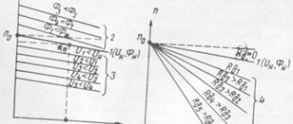
From equation (10) it follows that the mechanical characteristics in this mode at different resistor resistances in the armature circuit of the electric motor are a continuation of the characteristics of the motor mode in the region of the second quadrant (Fig. 7). With increasing speed w at constant R
the braking torque increases. An increase in the resistance of the external resistor in the armature circuit, with a constant negative static torque on the electric motor shaft, leads to an increase in the rotation speed of the drive.
Rice. 7 Fig. 8 |
The transition from the motor mode to the recuperation mode with a sharp increase in the engine excitation flux is shown in Fig. 8.
1. Familiarize yourself with the electrical equipment of the installation (see Fig. 9).
2. Calculate the resistance values of the braking resistors for the dynamic braking and back-on braking modes at I
/
I
H=2 and
I
/
I
H=2.5.
3. Remove and construct the mechanical characteristics of a DC electric motor with independent excitation:
a) natural;
b) artificial with additional resistors in the armature circuit of the electric motor with resistance R
1=5 Ohm and
R
2=10 Ohm;
c) artificial at excitation currents I
B=0.9
I
BH and
I
B=0.7
I
BH;
4. Take the characteristics of the electric motor:
a) for the mode of dynamic braking and back-on braking at the resistance of the braking resistors calculated in paragraph 2;
b) for regenerative braking mode with additional resistors in the motor armature circuit with resistance R
1=0 and
R
2=5 Ohm.
5. According to characteristics w = f
(
t
) and
I
I =
f
(
t
) calculate and plot the mechanical characteristics w (
M
) for all braking modes.
6. Using analytical formulas, calculate and construct natural and artificial mechanical characteristics w = f
(
M
) at
U=U
H and
R
I=5 Ohm.
| Type | R N, kW | U H, B | I H, A | R I, Om | n H, rpm |
| P22 | 1,0 | 220 | 5,9 | 4,17 | 1500 |
1. Before starting research, the resistance of the braking resistors is calculated using the equations:
— for dynamic braking mode
; (11)
- for back-off mode
, (12)
where R
Н=
U
H/
I
H - rated motor resistance;
w0= U
H/
K
.
2. When taking speed characteristics w = f
(
I
) in motor mode it is enough to get 3-4 points.
3. The speed characteristics of the engine in braking modes are calculated from the dependence diagrams w = f
(
t
) and
I
I =
f
(
t
), obtained using an oscilloscope.
Fig.9. Electrical schematic diagram of a laboratory installation |
When taking characteristics w = f
(
t
) and
I
I =
f
(
t
) in braking modes, it is necessary to turn on the engine under study, bring its rotation speed to the nominal value, set the required braking resistance, and for the regenerative braking mode, by weakening the excitation flow of the engine, bring its rotation speed to 2000 rpm , turn on the oscilloscope and press one of
buttons “DT”, “PV” or “RT”, depending on the operating mode for the duration of the transition process.
To transition from speed characteristics to mechanical ones, the relationship between current and torque is determined from equation (2). If the motor excitation current is different from the rated value, a new value should be determined, where C
is the value of the motor coefficient determined from equation (6).
The magnetization curve of the electric motor under study is shown in Fig. 10.
Self-excited braking
During self-excited braking, the field winding is not disconnected from the armature, but is switched using a control circuit so that the direction of the current in the field winding remains the same as in motor mode.
Circuit diagram of a series-excited DC motor for dynamic braking with self-excitation.
Characteristics of a series-excited DC motor during dynamic braking with self-excitation. Rext.3>Rext.2>Rext.1
For the emergence and existence of a self-excitation mode, it is necessary to satisfy such a condition as the presence of residual magnetism, and the flow of residual magnetism must coincide in direction with the main magnetic flux, which is why it is necessary to maintain the direction of the magnetic flux the same as it was in the motor mode.
Braking in the self-excitation mode occurs slower than in the independent excitation mode, since the braking characteristics are nonlinear.
Electric drive with DC motors (page 10)
Schemes with bypassing the armature of a series-excited DC motor are used to ensure low movement speeds, as well as to obtain a certain ideal no-load speed of a series-excited DC motor. Such circuits have found application in electric transport, electric drives of lifting machines and a number of other cases.
3.19. INHIBITION OF SEQUENTIAL EXCITATION DPT
For a series-excited DC DC, two options for the braking mode are possible: when the generator operates in series with the network (counter-switching braking mode) and independently of the network (dynamic braking mode).
Back braking
DPT of sequential excitation, as well as for DPT of independent excitation, can be implemented in two ways.
One of them is associated with a change in the polarity of the voltage on the armature winding while maintaining the same direction of the current in the field winding. At the same time, to limit the transient current, an additional resistor R
d is introduced into the DPT armature circuit.
As a result of these operations, the DPT (Fig. 381) will change from its natural characteristic 1
to characteristic
2,
section
b of
which corresponds to the back-on braking mode.
Braking by back-switching is also implemented in the case when the sequential excitation DC motor is loaded with active torque M
s exceeding the short circuit moment
M
k, z. Let's look at this method using Fig. 3.81.
Let us assume that the DBT in the original mode operates at point a
on characteristic
1
, overcoming the active load moment
M
s.
If now, without changing the polarity of the voltage on the DPT, an additional resistor R
d is introduced into its armature circuit, then the DPT will have a characteristic of the form
3
.
Since the torque of the DBT has become less than the load moment, it will first begin to slow down and then accelerate in the opposite direction, until at point d the
load moments
M
c and the DBT are equal. In this case, the engine will operate in reverse braking mode.
Dynamic braking
The sequential excitation DCT is implemented in two circuits for its inclusion.
In the first scheme (Fig. 3 82, a
) the excitation winding of the OD through an additional resistor
R
in is connected to a direct current source, and the armature winding is closed to the resistor
R
d. The result is a circuit typical for an independent excitation DPT, in which a series-excited DPT has the characteristics shown in Fig.
3.82, b
.
Specific to DBT of sequential excitation is dynamic inhibition with self-excitation, which is implemented according to the scheme in Fig. 3.83. For the emergence and existence of the self-excitation mode, the following conditions must be met: 1) the presence of residual magnetic flux in the DPT Fost; 2) coincidence in the direction of Fost and the magnetic flux F created by the excitation current; 3) closed armature circuit; 4) the speed of the DPT must be different from zero;
5) the EMF induced in the armature must be equal to the total voltage drop in the armature circuit resistors, i.e. E = IR
.
When these conditions are met, braking by self-excitation occurs as follows. Due to the presence of a residual magnetic field, when the armature rotates, an EMF is induced in it, under the influence of which a current flows through the armature and the excitation winding of the DPT. This current creates the main magnetic flux F, which, coinciding in direction with the residual flux Fost, will lead to an increase in EMF. This, in turn, will entail an increase in the current in the DPT, and this process of self-excitation of the DPT will continue until the EMF becomes equal to the total voltage drop in the armature circuit.
The static characteristics of the sequential excitation DC current in this mode can be obtained graphically using the condition E = IR
.
To do this, on one plane (Fig. 3.84, a
) the no-load characteristics
E( I ),
which are the dependence of the EMF of the machine on the excitation current at a fixed armature speed w=const, and the current-voltage characteristic of the armature circuit
IR ( I )
.
The intersection points of these characteristics correspond to the steady state for the given parameters of the DC armature circuit and its speed. So, with the total resistance of the armature circuit R
1, the points of the steady state are points
1
2 and 3, and with a different, higher resistance of the armature circuit
R
2
> R
1
-
points
4
and
5
.
If we now use the coordinates of these points of the steady state, namely the values of speed and current, then we can obtain the desired static electromechanical characteristics of the DC motor. In Fig. 3.84, b
This construction was carried out, as a result of which electromechanical characteristics were obtained for two accepted values of the total resistance of the armature circuit
R
1 and
R
2. The mechanical characteristics of a series-excited DC DC can be obtained from the electromechanical characteristics using universal characteristics.
Note that for the braking mode with self-excitation, there is a certain critical combination of parameters corresponding to the boundary of this mode. Such a critical combination in Fig. 3.84, a
with armature circuit resistance
R
1 the speed w4=wcr1 corresponds (with resistance
R
2
-
speed w3=wcr2). At lower speeds, self-excitation of the DPT does not occur.
The self-excited braking mode is used for intensive electric braking in electric drives of transport and lifting machines.
3.20.
CONTROL CIRCUIT OF SERIAL-EXCITATION DFC
Relay-contactor control circuits of series-excited DC motors during starting, reversing and braking are carried out according to the same principles of time, speed (EMF), current and path as for other types of DC motors. Many typical components that were discussed earlier can be used in an electric drive with a series-excited DC motor,
Let's consider the control circuit of a sequential excitation DC motor shown in Fig. 3.85 This circuit provides start-up of a DMT in two stages according to the time principle and reverse or braking by back-switching according to the EMF principle. The circuit includes five single-pole contactors KM, KM1, KM2, KMZ, KM4
;
two acceleration contactors KM5
and
KM6,
back-up contactor
KM7;
back-off relay
KVI
and
KV 2
;
time relay KT1
and
KT2;
switches
QF 1
and
QF 2.
The control element in the circuit is the command controller SA ,
having three positions: zero, “Forward” and “Back”.
Electric drive protection is provided by maximum relays KA1, KA2,
voltage relay
KV
and fuses
FA
.
The KVI
and
KV 2
back-off relays are configured in the same way as in the diagram in Fig. 3 45,
a
.
The start of the DPT, for example, in the conditional direction “Forward” is carried out by switching the command controller SA
to the “Forward” position If the protection is in the initial position, this will lead to the operation of the devices
KM, KM1, KM2
R
p and
R
arising due to the starting current
KT1
and
to turn on ,
which their contacts in the circuit of the
KM5
and
KM6
.
At the same time, the KVI
and with its contact will supply power to the
KM7 contactor.
The latter, when triggered, will short-circuit the back-off stage
R
p and at the same time the relay coil
KT1,
which, having lost power, will begin counting the time delay.
Next, in the manner discussed above for similar circuits, as a function of time, the starting resistor stages R
d1 and
R
d2 will be sequentially shorted.
For reverse command controller SA
is moved to the “Back” position.
When it moves to this position, the devices KM1, KM2, KM7, KM5, KM6 are turned off,
introducing resistors
R
p,
R
d1,
R
d2 into the armature circuit and thereby preparing the DPT for reverse or braking
When you next turn on the devices KM, KM2, KM4
The polarity of the voltage on the DPT armature changes, and it goes into the back-switching braking mode.
In accordance with its setting, relay KV 2,
despite the closure of the
KM3
in its power circuit, does not operate, as a result of which the contactors
KM7, KM5
and
KM6
R
p +
R
d1 +
R
fully inserted into the armature circuit .
As the speed decreases, the voltage on the relay coil K V 2
(see Fig. 346,
b
), and at a speed close to zero, it will operate. If the controller remains in the “Back” position, then the process of running the DC motor in this direction begins with the order of operation of the circuit discussed above.
If, when reaching zero speed, the controller is moved to the middle position, the DPT will be disconnected from the network and the circuit will return to its original position.
In general, accurate analysis of transient processes in an electric drive with a sequential excitation DC motor and obtaining the dependence of coordinate changes over time are complex tasks. This is determined by the fact that the differential equations for the armature circuit of the motor and the mechanical part of the drive are nonlinear due to the presence in them of the product of two variables - current and magnetic flux for torque and speed and flux for EMF. An additional complication of the study is associated with the nonlinear dependence of the magnetic flux on the current, expressed by the magnetization curve, as well as the nonlinearity of the characteristics of the DCT. In this regard, an accurate study of transient processes in an electric drive is possible only with the help of computers. In practical engineering calculations, as a rule, various approximate methods are used to obtain transient process curves
3.21.
CONNECTION DIAGRAM AND CHARACTERISTICS OF MIXED-EXCITATION DSC
The main connection circuit of mixed-excitation DSC is shown in Fig. 3.86, a
.
The motor has two excitation windings - a serial ORP
connected in series with the armature, and an independent
ORV
.
As a result, the magnetic flux of the DPT is the sum of two components - the flux Fo, in, n, created by the OVP,
and the flux Fo, in, p, created by
the ORP
.
The dependence of both components and the total flow of DPT F as a function of current is shown in Fig. 3.86, b
respectively, in the form of dashed lines
1
and
2
and solid line
3
.
It is important to note that when the armature current tends to the value – I
1
,
the magnetic flux Ф tends to zero, i.e. the DCT is demagnetized.
The electromechanical and mechanical characteristics of a mixed-excitation DC DC are expressed respectively by formulas (3.163) and (3.164), in which the magnetic flux Ф is also a function of the current.
To obtain areas of characteristics for w>w0 (second quadrant), we will carry out the following additional analysis.
1 At I
®-
I
1 (see Fig. 3.86,
b
) magnetic flux
Ф
®
0
and according to (3.163) w®¥.
Thus, the vertical line corresponding to the current value I
= -
I
1 is an asymptote of the electromechanical characteristic, the form of which is shown in Fig. 3.87,
a
.
2
The mechanical characteristic of a mixed-excitation DC DC in the second quadrant can be obtained by considering the formula for the electromagnetic torque of a DC DC DC (3.3). It follows from it that when
I
® -
I
1
Ф
®
0
and w®¥, the torque of the DC DC tends to zero.
In other words, the velocity axis is an asymptote of the mechanical characteristic. Since at w=w0 M=0,
then at the speed interval w0
Mmax
, and the mechanical characteristic has the form of a curve shown in Fig.
3.87, b
.
A mixed excitation motor, having two excitation windings, combines the properties of both independent excitation DFC and sequential excitation DFC.
The mixed excitation motor can operate in all possible modes, namely as a motor, a generator in parallel, in series and independently of the network, as well as in idle and short circuit modes.
Regulation of the coordinates of a mixed-excitation DC DC can be carried out by all methods characteristic of a DC DC associated with changes in the magnetic flux, voltage and resistor resistance in the armature circuit.
The mixed excitation DC motor control is carried out using the circuits considered in relation to the independent and sequential excitation DC motors.
Note that due to the relatively low technical and economic indicators of a mixed-excitation DC motor (high cost, increased weight, dimensions and material consumption), an electric drive with a mixed-excitation DC motor is used relatively rarely.
| Due to the large volume, this material is placed on several pages: 10 |