Considering signals and types of signals, it must be said that there are different amounts of these connections. Every day, every person encounters the use of an electronic device. No one can imagine modern life without them. We are talking about the operation of a TV, radio, computer, and so on. Previously, no one thought about what signal is used in many operational devices. Now the words analog, digital and discrete have long been heard.
Not all, but some of the above signals are considered to be quite high quality and reliable. Digital transmission has not been used for as long as analogue. This is due to the fact that technology began to support this type only recently; this type of signal was also discovered relatively not so long ago. Every person encounters discreteness all the time. Speaking of signal processing types, it is necessary to recall that this one is a little intermittent.
If we delve deeper into science, it should be said that the transmission of information is discrete, which allows you to transfer data and change the time of the environment. Thanks to the last property, a discrete signal can take on any value. At the moment, this indicator is fading into the background, after most equipment began to be produced on chips.
Digital and other signals are integral, components interact with each other 100%. In discreteness, the opposite is true. The fact is that here each part works independently and is responsible for its functions separately.
Signal
Let's look at the types of communication signals a little later, but now you should get acquainted with what the signal itself is, in principle. This is a common code that is transmitted over the air by systems. This is a general type of formulation.
In the field of information and some other technologies, there is a special medium that allows messages to be transmitted. It can be created, but it cannot be accepted. In principle, some systems may accept it, but this is not required. If the signal is considered a message, then it is necessary to “catch” it.
Such a data transfer code can be called a regular mathematical function. It describes any change to the available parameters. If we consider radio engineering theory, it should be said that such options are considered basic. It should be noted that the concept of “noise” is similar to a signal.
It distorts it, can overlap with already transmitted code, and also represents a function of time itself. The article will describe signals and types of signals below; we are talking about discrete, analog and digital. Let's briefly consider the entire theory on the topic.
Periodic signals
Periodic signals are the most common because they include sine waves. The alternating current in the outlet at home is a sinusoid, changing smoothly over time with a frequency of 50 Hz.
The time that passes between individual repetitions of a sinusoid cycle is called its period. In other words, this is the time it takes for the signal to start repeating.
The period can vary from fractions of a second to thousands of seconds, as it is related to its frequency. For example, a sine wave that takes 1 second to complete a cycle has a period of one second. Likewise, a sine wave that takes 5 seconds to complete a cycle has a period of 5 seconds, and so on.
So, the length of time it takes for a signal to complete a full cycle of its change before it repeats again is called the period of the signal and is measured in seconds. We can express the signal as the number of cycles T per second as shown in the figure below.
Types of signals
There are several types, as well as classifications of existing signals. Let's look at them.
The first type is an electrical signal, there are also optical, electromagnetic and acoustic. There are several other similar types, but they are not popular. This classification occurs according to the physical environment.
According to the method of setting the signal, they are divided into regular and irregular. The first type has an analytical function, as well as a deterministic type of data transfer. Random signals can be generated using some theories from higher mathematics, moreover, they are capable of taking on many values in completely different periods of time.
The types of signal transmission are quite different; it should be noted that signals according to this classification are divided into analog, discrete and digital. Often these signals are used to ensure the operation of electrical appliances. In order to understand each of the options, you need to remember the school physics course and read a little theory.
Square wave
Rectangular signals differ from meanders in that the durations of the positive and negative parts of the period are not equal. Square wave signals are therefore classified as single-ended signals.
In this case, I have depicted a signal that takes only positive values, although, in general, negative signal values can be significantly below the zero mark.
In the example shown, the duration of the positive pulse is longer than the duration of the negative one, although this is not necessary. The main thing is that the signal shape is rectangular.
Signal repetition period ratio
*** QuickLaTeX cannot compile formula: T *** Error message: Cannot connect to QuickLaTeX server: SSL certificate problem: certificate has expired Please make sure your server/PHP settings allow HTTP requests to external resources (“allow_url_fopen”, etc.) These links might help in finding a solution: https://wordpress.org/extend/plugins/core-control/ https://wordpress.org/support/topic/an-unexpected-http-error-occurred-during-the- api-request-on-wordpress-3?replies=37 , to the duration of the positive pulse *** QuickLaTeX cannot compile formula: \tau *** Error message: Cannot connect to QuickLaTeX server: SSL certificate problem: certificate has expired Please make sure your server/PHP settings allow HTTP requests to external resources (“allow_url_fopen”, etc.) These links might help in finding a solution: https://wordpress.org/extend/plugins/core-control/ https://wordpress.org /support/topic/an-unexpected-http-error-occurred-during-the-api-request-on-wordpress-3?replies=37
, is called duty cycle:
*** QuickLaTeX cannot compile formula: \ *** Error message: Cannot connect to QuickLaTeX server: SSL certificate problem: certificate has expired Please make sure your server/PHP settings allow HTTP requests to external resources (“allow_url_fopen”, etc.) These links might help in finding a solution: https://wordpress.org/extend/plugins/core-control/ https://wordpress.org/support/topic/an-unexpected-http-error-occurred-during-the- api-request-on-wordpress-3?replies=37
The reverse duty cycle value is called the duty cycle:
*** QuickLaTeX cannot compile formula: \ *** Error message: Cannot connect to QuickLaTeX server: SSL certificate problem: certificate has expired Please make sure your server/PHP settings allow HTTP requests to external resources (“allow_url_fopen”, etc.) These links might help in finding a solution: https://wordpress.org/extend/plugins/core-control/ https://wordpress.org/support/topic/an-unexpected-http-error-occurred-during-the- api-request-on-wordpress-3?replies=37
Calculation example
Let there be a rectangular signal with a pulse duration of 10 ms and a duty cycle of 25%. It is necessary to find the frequency of this signal.
The duty cycle is 25% or ¼, and coincides with the pulse width, which is 10ms. Thus, the signal period should be equal to: 10ms (25%) + 30ms (75%) = 40ms (100%).
*** QuickLaTeX cannot compile formula: f = \frac{1}{T} = \frac{1}{(10 + 30) \cdot 10^{-3}c} = 25 *** Error message: Cannot connect to QuickLaTeX server: SSL certificate problem: certificate has expired Please make sure your server/PHP settings allow HTTP requests to external resources (“allow_url_fopen”, etc.) These links might help in finding a solution: https://wordpress.org/extend /plugins/core-control/ https://wordpress.org/support/topic/an-unexpected-http-error-occurred-during-the-api-request-on-wordpress-3?replies=37
Hz
Square wave signals can be used to control the amount of power delivered to a load, such as a lamp or motor, by varying the duty cycle of the signal. The higher the duty cycle, the greater the average amount of energy must be supplied to the load, and, accordingly, a lower duty cycle means a lower average amount of energy supplied to the load. A great example of this is the use of pulse width modulation in speed controllers. The term pulse width modulation (PWM) literally means “change in pulse width.”
Why is the signal processed?
The signal must be processed in order to obtain the information that is encrypted in it. If we consider the types of signal modulation, it should be noted that in terms of amplitude and frequency shift keying, this is a rather complex process that must be fully understood. Once the information is obtained, it can be used in completely different ways. In some situations, it is formatted and sent further.
It is also worth noting other reasons why signal processing occurs. It consists in compressing the frequencies that are transmitted, but without damaging all the information. Then it is formatted again and transmitted. This is done at slow speeds. If we talk about analog and digital signals, then special methods are used here. There is filtering, convolution and some other functions. They are needed to restore information if the signal is damaged.
What is a signal
A signal is a certain physical process whose parameters change in accordance with the transmitted message. Example - an electrical signal, a radio signal, as a special case of an electromagnetic signal, an acoustic signal, an optical signal, etc. Depending on the environment in which the signal is propagating. A signal is a material carrier of information.
Usually a signal, regardless of its physical nature, is represented as some function of time x(t) . This representation is a generally accepted mathematical abstraction of a physical signal.
Signal types
- Deterministic, or regular, is a signal whose law of change is known and all its parameters are known.
Does this signal convey information? Information reduces uncertainty. In a deterministic signal we know everything, we know what it will be like in a minute, in a year. A deterministic signal does not contain any information. For example, a signal from a local oscillator, we generated it ourselves, set the frequency, amplitude, and phase.
- Quasi-deterministic is a signal whose law of variation is known, but one or more parameters are a random variable.
Example: x(t)=Asin(wt+j), where amplitude A and j are random variables.
For example, we know its frequency, but we do not know the amplitude and phase - this is a quasi-deterministic signal, a “quasi” - almost, almost certain signal. The information introduces some randomness. If we know the amplitude, frequency and phase, then the information is not there. A quasi-deterministic signal transmits information; the information is transmitted in those parameters that are random; in our example, the amplitude and phase are random variables. It is in these quantities that information is transmitted. Information always carries chaos and randomness. All modulated signals, FM, PM, are quasi-deterministic signals.
- A signal is called random, the instantaneous values of which are not known, but can only be predicted with some probability.
In addition, all signals can be continuous (analog) or discrete (digital or pulse).
We can judge a random signal by its probabilistic characteristics. We can know its probability density, but we don’t know what value the signal will take in a second or a minute. When we work with a random signal, we always work with probability.
Signal parameters
What parameters will we use? This is the energy over a certain time interval T. X(t) is the signal itself, to determine the energy we must take it modulo, square it, integrate over a certain period of time and get the energy.
Average power over some time t. This is energy divided by time.
Instantaneous power, if average power is measured over a certain period of time, then instantaneous power is measured at one specific moment in time.
Average power is measured over a period of time, and instantaneous power at a point.
Spectral energy and power density
The spectral density of a signal characterizes the distribution of signal energy or power over a frequency range. Spectral energy density is how our energy is distributed across the frequency range. Calculated through the Fourier transform.
And accordingly, PSD is how we distribute power across the frequency range.
In the formula, the modulus squared is the spectral energy density, divided by time T and, by definition, time T should tend to infinity. But in practice, no one waits for infinity; everyone evaluates the PSD over a certain time interval.
PSD is a frequency-dependent function. On the PSD scale, we take 10 W/Hz, and the vicinity of 1 Hz in frequency. Then in the 1 Hz band there will be 10 W of power.
There are two signals and their power spectral densities are presented. QUESTION. Which signal has more power?
We must determine the area under the curve and integrate. S1=2*10=20 W, S2=1*30=30 W. In the first case, S1 has a power of 20 W, and in the second, 30 W.
PSD of the real signal, displayed on the spectrum analyzer.
Modern spectrum analyzers can automatically calculate the area; you enable power detection, set the frequency interval in which it should measure this power, and it itself calculates the channel signal power.
Creation and formatting
Many types of information signals that we will talk about in the article need to be created and then formatted. To do this, you must have a digital-to-analog converter, as well as an analog-to-digital converter. As a rule, they are both used in the same situation: only in the case of using a technique such as DSP.
In other cases, only the first device will do. In order to create physical analog codes and then reformat them into digital methods, it is necessary to use special devices. This will prevent damage to information as much as possible.
Dynamic range
The range of any type of analog signal is easy to calculate. It is necessary to use the difference between higher and lower volume levels, which is shown in decibels.
It should be noted that the information depends entirely on the characteristics of its execution. Moreover, we are talking about both music and the conversations of ordinary people. If we take an announcer who will read the news, then his dynamic range will be no more than 30 decibels. And if you read any work in color, then this figure will increase to 50.
Analog signal
The types of presentation of the satisfied signal are different. It should be noted that the analog signal is continuous. If we talk about the disadvantages, many note the presence of noise, which can, unfortunately, lead to loss of information.
Quite often a situation arises where it is unclear where in the code there is really important information and where there are simply distortions. It is because of this that the analog signal has become less popular, and at the moment it is being replaced by digital technology.
Digital signal
It should be noted that such a signal, like other types of signals, is a data stream that is described by discrete characteristics.
It should be noted that its amplitude can be repeated. If the analogue version described above is capable of arriving at the end point with a huge amount of noise, then the digital version does not allow this. It is able to independently eliminate most of the interference in order to avoid damage to information. It should also be noted that this type conveys information without any semantic loads.
Thus, a user can easily send multiple messages through one physical channel. It should be noted that, unlike the types of sound signal that are the most common at the moment, as well as analog, digital is not divided into several types. He is unique and independent. Represents a binary stream. Now it is quite popular, it is easy to use, as evidenced by reviews.
Sine wave
Period time is often measured in seconds (s), milliseconds (ms), and microseconds (µs).
For a sine waveform, the time period of the signal can also be expressed in degrees, or in radians, given that one complete cycle is equal to 360° (T = 360°), or, if in radians, then
*** QuickLaTeX cannot compile formula: 2 \pi *** Error message: Cannot connect to QuickLaTeX server: SSL certificate problem: certificate has expired Please make sure your server/PHP settings allow HTTP requests to external resources (“allow_url_fopen”, etc .) These links might help in finding a solution: https://wordpress.org/extend/plugins/core-control/ https://wordpress.org/support/topic/an-unexpected-http-error-occurred-during- the-api-request-on-wordpress-3?replies=37 (T = *** QuickLaTeX cannot compile formula: 2 \pi *** Error message: Cannot connect to QuickLaTeX server: SSL certificate problem: certificate has expired Please make make sure your server/PHP settings allow HTTP requests to external resources (“allow_url_fopen”, etc.) These links might help in finding a solution: https://wordpress.org/extend/plugins/core-control/ https://wordpress. org/support/topic/an-unexpected-http-error-occurred-during-the-api-request-on-wordpress-3?replies=37
).
Period and frequency are mathematically the reciprocals of each other. As the signal period time decreases, its frequency increases and vice versa.
The relationship between the signal period and its frequency:
*** QuickLaTeX cannot compile formula: f = \frac{1}{T} *** Error message: Cannot connect to QuickLaTeX server: SSL certificate problem: certificate has expired Please make sure your server/PHP settings allow HTTP requests to external resources (“allow_url_fopen”, etc.) These links might help in finding a solution: https://wordpress.org/extend/plugins/core-control/ https://wordpress.org/support/topic/an-unexpected-http -error-occurred-during-the-api-request-on-wordpress-3?replies=37
Hz
*** QuickLaTeX cannot compile formula: T = \frac{1}{f} *** Error message: Cannot connect to QuickLaTeX server: SSL certificate problem: certificate has expired Please make sure your server/PHP settings allow HTTP requests to external resources (“allow_url_fopen”, etc.) These links might help in finding a solution: https://wordpress.org/extend/plugins/core-control/ https://wordpress.org/support/topic/an-unexpected-http -error-occurred-during-the-api-request-on-wordpress-3?replies=37
c
One hertz is exactly equal to one cycle per second, but one hertz is a very small value, so you often see prefixes indicating the order of magnitude of the signal, such as kHz, MHz, GHz and even THz
| Prefix | Definition | Record | Period |
| Kilo | thousand | kHz | 1 ms |
| Mega | million | MHz | 1 µs |
| Giga | billion | GHz | 1 ns |
| Tera | trillion | THz | 1 ps |
Application of digital signal
Considering the types of signal transmission, it is necessary to say where the digital option is used. How does it differ from many others in transmission and use? The fact is that upon entering the repeater, it is completely regenerated.
When the equipment receives a signal that has received noise and interference during transmission, it is immediately formatted. Thanks to this, TV towers can regenerate the signal, avoiding the use of noise effect.
In this case, analog communication will be much better, since when receiving information with a large amount of distortion, it can be extracted at least partially. If we talk about the digital version, then this is impossible. If more than 50% of the signal has noise, then we can assume that the information is completely lost.
Many people, discussing cellular communications, of completely different formats and transmission methods, said that sometimes it is almost impossible to talk. People may not hear words or phrases. This can only happen on a digital line if there is noise.
If we talk about analog communications, then in this case the conversation can be continued further. Due to such problems, repeaters always generate a new signal in order to reduce gaps.
Ramp signal
A ramp wave is another type of periodic waveform. As the name suggests, the shape of this signal resembles the teeth of a saw. A sawtooth signal can be a mirror image of itself, having either a slow rise but a very steep fall, or an extremely steep, nearly vertical rise and a slow fall.
The slow-rising ramp wave is the more common of the two waveform types, being almost perfectly linear. The sawtooth waveform is generated by most function generators and consists of a fundamental frequency (f) and even harmonics. This means, from a practical point of view, that it is rich in harmonics, and in the case of, for example, music synthesizers, produces high-quality sound without distortion for musicians.
Discrete signal
Currently, a person uses various dialers or other electronic devices that receive signals. The types of signals are quite diverse, and one of them is discrete. It should be noted that in order for such devices to work, it is necessary to transmit an audio signal. That is why a channel is needed that has a much higher level of throughput than was previously described.
What is this connected with? The fact is that in order to transmit quality sound, it is necessary to use a discrete signal. It does not create a wave of sound, but a digital copy of it. Accordingly, the transmission comes from the technology itself. The advantages of such a transfer are that batch sending will be carried out in batches, and the amount of transmitted data will be reduced.
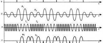
Harmonic vibrations
There were several articles on the hub on the Fourier transform and about all sorts of beauties such as Digital Signal Processing (DSP), but it is completely unclear to the inexperienced user why all this is needed and where, and most importantly, how to apply it.
Frequency response of noise.
Personally, after reading these articles (for example, this one), it did not become clear to me what it was and why it was needed in real life, although it was interesting and beautiful. I want to not just look at beautiful pictures, but, so to speak, to feel in my gut what and how it works. And I will give a specific example with the generation and processing of sound files. It will be possible to listen to the sound, and look at its spectrum, and understand why this is so. The article will not be of interest to those who know the theory of functions of a complex variable, DSP and other scary topics. It is more for the curious, schoolchildren, students and those who sympathize with them :).
Let me make a reservation right away: I am not a mathematician, and I may even say many things incorrectly (correct them with a personal message), and I am writing this article based on my own experience and my own understanding of current processes. If you're ready, let's go.
A few words about materiel
If we remember our school mathematics course, we used a circle to plot the sine graph. In general, it turns out that rotational motion can be turned into a sine wave (like any harmonic oscillation). The best illustration of this process is given in Wikipedia
Harmonic vibrations
Those. in fact, the sine graph is obtained from the rotation of the vector, which is described by the formula:
f(x) = A sin (ωt + φ),
where A is the length of the vector (oscillation amplitude), φ is the initial angle (phase) of the vector at zero time, ω is the angular velocity of rotation, which is equal to:
ω=2 πf, where f is the frequency in Hertz.
As we see, knowing the signal frequency, amplitude and angle, we can construct a harmonic signal.
The magic begins when it turns out that the representation of absolutely any signal can be represented as a sum (often infinite) of different sinusoids. In other words, in the form of a Fourier series. I will give an example from the English Wikipedia. Let's take a sawtooth signal as an example.
Ramp signal
Its amount will be represented by the following formula:
If we add up one by one, take first n=1, then n=2, etc., we will see how our harmonic sinusoidal signal gradually turns into a saw:
This is probably most beautifully illustrated by one program I found on the Internet. It was already said above that the sine graph is a projection of a rotating vector, but what about more complex signals? This, oddly enough, is a projection of many rotating vectors, or rather their sum, and it all looks like this:
Vector drawing saw.
In general, I recommend going to the link yourself and trying to play with the parameters yourself and see how the signal changes. IMHO I have never seen a more visual toy for understanding.
It should also be noted that there is an inverse procedure that allows you to obtain frequency, amplitude and initial phase (angle) from a given signal, which is called the Fourier Transform.
Fourier series expansion of some well-known periodic functions (from here)
I won’t dwell on it in detail, but I will show how it can be applied in life. In the bibliography I will recommend where you can read more about the materiel.
Let's move on to practical exercises!
It seems to me that every student asks a question while sitting at a lecture, for example on mathematics: why do I need all this nonsense? And as a rule, having not found an answer in the foreseeable future, unfortunately, he loses interest in the subject. Therefore, I will immediately show the practical application of this knowledge, and you will already master this knowledge yourself :).
I will implement everything further on my own. I did everything, of course, under Linux, but did not use any specifics; in theory, the program will compile and run under other platforms.
First, let's write a program to generate an audio file. The wav file was taken as the simplest one. You can read about its structure here. In short, the structure of a wav file is described as follows: a header that describes the file format, and then there is (in our case) an array of 16-bit data (pointer) with a length of: sampling_frequency*t seconds or 44100*t pieces.
An example was taken here to generate a sound file. I modified it a little, corrected errors, and the final version with my edits is now on Github here
github.com/dlinyj/generate_wav
Let's generate a two-second sound file with a pure sine wave with a frequency of 100 Hz. To do this, we modify the program as follows:
#define S_RATE (44100) //sampling frequency #define BUF_SIZE (S_RATE*10) /* 2 second buffer */ …. int main(int argc, char * argv[]) { ... float amplitude = 32000; //take the maximum possible amplitude float freq_Hz = 100; //signal frequency /* fill buffer with a sine wave */ for (i=0; i
Please note that the formula for pure sine corresponds to the one we discussed above. The amplitude of 32000 (32767 could have been taken) corresponds to the value that a 16-bit number can take (from minus 32767 to plus 32767).
As a result, we get the following file (you can even listen to it with any sound reproducing program). Let's open this audacity file and see that the signal graph actually corresponds to a pure sine wave:
Pure tube sine
Let's look at the spectrum of this sine (Analysis->Plot spectrum)
Spectrum graph
A clear peak is visible at 100 Hz (logarithmic scale). What is spectrum? This is the amplitude-frequency characteristic. There is also a phase-frequency characteristic. If you remember, I said above that to build a signal you need to know its frequency, amplitude and phase? So, you can get these parameters from the signal. In this case, we have a graph of frequencies corresponding to amplitude, and the amplitude is not in real units, but in Decibels.
A value expressed in decibels is numerically equal to the decimal logarithm of the dimensionless ratio of a physical quantity to the physical quantity of the same name, taken as the original, multiplied by ten.
In this case, simply the logarithm of the amplitude multiplied by 10. The logarithmic scale is convenient to use when working with signals.
To be honest, I don’t really like the spectrum analyzer in this program, so I decided to write my own with blackjack and whores, especially since it’s not difficult.
We are writing our own spectrum analyzer
This might get boring, so you can skip straight to the next chapter.
Since I understand perfectly well that there is no point in posting foot wraps of code here, those who are really interested will find it and dig into it themselves, and those who are not interested will be bored, I will only focus on the main points of writing a spectrum analyzer for a wav file.
First, we need to read the wav file. There you need to read the header to understand what the file contains. I did not implement a sea of options for reading this file, but settled on only one. The file reading example was taken from here with virtually no changes, IMHO it’s an excellent example. There is also an implementation in Python.
The next thing we need is a fast Fourier transform. This is the same transformation that allows you to obtain a vector a
original signals. Don’t let this scare you for now, I’ll explain later. Again, I didn’t reinvent the wheel, but took a ready-made example from here.
I understand that in order to explain how the program works, it is necessary to explain what the fast Fourier transform is, and this is at least one more article.
First, let's allocate the arrays:
c = calloc(size_array*2, sizeof(float)); // array of rotation factors in = calloc(size_array*2, sizeof(float)); //input array out = calloc(size_array*2, sizeof(float)); //output array
Let me just say that in the program we read data into an array of length size_array (which we take from the header of the wav file).
while( fread(&value,sizeof(value),1,wav) ) { in[j]=(float)value; j+=2; if (j > 2*size_array) break; }
The array for fast Fourier transform must be a sequence {re[0], im[0], re[1], im[1],… re[fft_size-1], im[fft_size-1]}, where fft_size=1 << p — number of FFT points. I’ll explain it in normal language: this is an array of complex numbers. I’m even afraid to imagine where the complex Fourier transform is used, but in our case, our imaginary part is equal to zero, and the real part is equal to the value of each point of the array. Another feature of the fast Fourier transform is that it calculates arrays that are multiples only of powers of two. As a result, we must calculate the minimum power of two:
int p2=(int)(log2(header.bytes_in_data/header.bytes_by_capture));
The logarithm of the number of bytes in the data divided by the number of bytes at one point.
After this, we calculate the rotation factors:
fft_make(p2,c); // function for calculating rotation factors for FFT (the first parameter is a power of two, the second is an allocated array of rotation factors).
And we feed our just array into the Fourier transformer:
fft_calc(p2, c, in, out, 1); //(one means we are getting a normalized array).
At the output we get complex numbers of the form {re[0], im[0], re[1], im[1],... re[fft_size-1], im[fft_size-1]}. For those who don’t know what a complex number is, I’ll explain. It’s not for nothing that I started this article with a bunch of rotating vectors and a bunch of GIFs. So, a vector on the complex plane is determined by the real coordinate a1 and the imaginary coordinate a2. Or length (this is amplitude Am for us) and angle Psi (phase).
Vector on the complex plane
Please note that size_array=2^p2. The first point of the array corresponds to a frequency of 0 Hz (constant), the last point corresponds to the sampling frequency, namely 44100 Hz. As a result, we must calculate the frequency corresponding to each point, which will differ by the delta frequency:
double delta=((float)header.frequency)/(float)size_array; //sampling frequency per array size.
Allocation of the amplitude array:
double * ampl; ampl = calloc(size_array*2, sizeof(double));
And look at the picture: amplitude is the length of the vector. And we have its projections onto the real and imaginary axis. As a result, we will have a right triangle, and here we remember the Pythagorean theorem, and count the length of each vector, and immediately write it into a text file:
for(i=0;i<(size_array);i+=2) { fprintf(logfile,"%.6f %f\n",cur_freq, (sqrt(out
*out +out[i+1]*out[i +1])));
cur_freq+=delta; } As a result, we get a file that looks something like this: ... 11.439514 10.943008 11.607742 56.649738 11.775970 15.652428 11.944199 21.872342 12.112427 30.635371 12.280655 30 .329171 12.448883 11.932371 12.617111 20.777617 ... The final version of the program lives on GitHub here: github.com/dlinyj/fft
Let's try!
Now we feed the resulting program that sine sound file
./fft_an ../generate_wav/sin\ 100\ Hz.wav format: 16 bits, PCM uncompressed, channel 1, freq 44100, 88200 bytes per sec, 2 bytes by capture, 2 bits per sample, 882000 bytes in data chunk= 441000 log2=18 size array=262144 wav format Max Freq = 99.928 , amp =7216.136
And we get a text file of the frequency response. We build its graph using a gnuplot
Script for construction:
#! /usr/bin/gnuplot -persist set terminal postscript eps enhanced color solid set output "result.ps" #set terminal png size 800, 600 #set output "result.png" set grid xtics ytics set log xy set xlabel "Freq, Hz" set ylabel "Amp, dB" set xrange [1:22050] #set yrange [0.00001:100000] plot "test.txt" using 1:2 title "AFC" with lines linestyle 1
Please note the limitation in the script on the number of points in X: set xrange [1:22050]. Our sampling frequency is 44100, and if we recall Kotelnikov’s theorem, then the signal frequency cannot be higher than half the sampling frequency, therefore we are not interested in a signal above 22050 Hz. Why this is so, I advise you to read in specialized literature. So (drumroll), run the script and see:
Spectrum of our signal
Note the sharp peak at 100 Hz. Don't forget that the axes are on a logarithmic scale! The wool on the right is what I think are Fourier transform errors (windows come to mind here).
Let's indulge?
Come on! Let's look at the spectra of other signals!
There is noise around...
First, let's plot the noise spectrum.
The topic is about noise, random signals, etc. worthy of a separate course. But we will touch on it lightly. Let's modify our wav file generation program and add one procedure: double d_random(double min, double max) { return min + (max - min) / RAND_MAX * rand(); } it will generate a random number in the given range. As a result, main will look like this:
int main(int argc, char * argv[]) { int i; float amplitude = 32000; srand((unsigned int)time(0)); //initialize the random number generator for (i=0; i
Let's generate a file (I recommend listening to it). Let's look at it in audacity.
Signal in audacity
Let's look at the spectrum in the audacity program.
Range
And let's look at the spectrum using our program:
Our spectrum
I would like to draw your attention to a very interesting fact and feature of noise - it contains the spectra of all harmonics. As can be seen from the graph, the spectrum is quite even. Typically, white noise is used for frequency analysis of bandwidth, such as audio equipment. There are other types of noise: pink, blue and others
. Homework is to find out how they differ.
What about compote?
Now let's look at another interesting signal - a meander. I gave above a table of expansions of various signals in Fourier series, you look at how the meander is expanded, write it down on a piece of paper, and we will continue.
To generate a square wave with a frequency of 25 Hz, we once again modify our wav file generator:
int main(int argc, char * argv[]) { int i; short int meandr_value=32767; /* fill buffer with a sine wave */ for (i=0; i
As a result, we get an audio file (again, I advise you to listen), which you should immediately watch in audacity
His Majesty is the meander or meander of a healthy person
Let's not languish and look at its spectrum:
Meander spectrum
It’s not very clear yet what it is... Let’s take a look at the first few harmonics:
First harmonics
It's a completely different matter! Well, let's look at the sign. Look, we only have 1, 3, 5, etc., i.e. odd harmonics. We see that our first harmonic is 25 Hz, the next (third) is 75 Hz, then 125 Hz, etc., while our amplitude gradually decreases. Theory meets practice! Now attention! In real life, a square wave signal has an infinite sum of harmonics of higher and higher frequencies, but as a rule, real electrical circuits cannot pass frequencies above a certain frequency (due to the inductance and capacitance of the tracks). As a result, you can often see the following signal on the oscilloscope screen:
Smoker's meander
This picture is just like the picture from Wikipedia, where for the example of a meander, not all frequencies are taken, but only the first few.
The sum of the first harmonics, and how the signal changes
The meander is also actively used in radio engineering (it must be said that this is the basis of all digital technology), and it is worth understanding that with long circuits it can be filtered so that the mother does not recognize it. It is also used to check the frequency response of various devices. Another interesting fact is that TV jammers worked precisely on the principle of higher harmonics, when the microcircuit itself generated a meander of tens of MHz, and its higher harmonics could have frequencies of hundreds of MHz, exactly at the operating frequency of the TV, and the higher harmonics successfully jammed the TV broadcast signal.
In general, the topic of such experiments is endless, and you can now continue it yourself.
Reading Suggestions
Book
For those who don’t understand what we’re doing here, or vice versa, for those who understand but want to understand it even better, as well as for students studying DSP, I highly recommend this book. This is a DSP for dummies, which is the author of this post. There, complex concepts are explained in a language accessible even to a child.
Conclusion
In conclusion, I would like to say that mathematics is the queen of sciences, but without real application, many people lose interest in it. I hope this post will encourage you to study such a wonderful subject as signal processing, and analog circuitry in general (plug your ears so your brains don’t leak out!). Good luck!
Types of modulation
While describing the types of signals and signals in general, it is also necessary to talk about modulation. What it is? This is the process of changing several vibration parameters at once, which are carried out according to a certain law. It should be noted that modulation is divided into digital and pulse, as well as some others.
In turn, many of them are divided separately into several types, and there are quite a lot of them. It should be said about the main characteristics of this concept. For example, due to the types of signal modulation, it is possible to achieve stable transmission and minimal loss, but it should be noted that each of them requires a special linearity amplifier.