Basic methods for calculating electrical loads
— By rated power and utilization factor;
— By rated power and demand factor;
— By average power and design coefficient;
— By average power and deviation of the calculated load from the average;
— By average power and load curve shape factor.
The use of a particular method is determined by the permissible error of calculations and the availability of initial data.
Method for calculating electrical loads based on rated power and utilization factor
The method for determining design loads based on rated power and utilization factor is used, as a rule, for individual electric power plants with voltages up to 1 kV, operating in long-term mode (PV = 1).
According to this method, the design loads are assumed to be equal to the average load values for the busiest shift:
— calculated active power consumed by one electric unit, in the presence of a load schedule for active power
, (5.1)
where is the estimated active power, kW; – average value of active power of the electric unit for the busiest shift, kW;
— calculated active power consumed by one electric unit, in the absence of a load schedule for active power
, (5.2)
where is the coefficient of active power utilization by the electrical receiver for the period of time under consideration (technological parameter);
– rated active power of the electric unit, kW;
— calculated reactive power consumed by one electric unit, in the presence of a load schedule for reactive power
, (5.3)
where is the calculated reactive power, kVAr; – average value of reactive power of the electric unit for the busiest shift, kVAr;
— calculated reactive power consumed by one electric unit, in the absence of a load schedule for reactive power
, (5.4)
where is the coefficient of utilization of reactive power of the electric power plant for the period of time under consideration (technological parameter); – rated reactive power of the electric unit, kW; tg is the rated value of the reactive power factor corresponding to cosEP;
— estimated total power consumed by one electric unit:
, (5.5)
where is the calculated value of the total power of the electric unit, kVA;
— calculated value of the electric current
, (5.6)
where is the design current of the electric current, A; – power supply voltage, kV.
Using this method, it is possible to determine the design loads of a group of electric drives with voltages up to 1 kV, connected by a technological process (for example, multi-motor drives), and their number, as a rule, is no more than three or four. The operating mode of electrical receivers of this group must be reduced to a long-term mode (PV = 1).
Design loads of the ED group determined by this method:
— calculated active power consumed by a group of electric power plants, in the presence of a group load node graph for active power
, (5.7)
where is the estimated active power consumed by the electric group, kW;
– average active power consumed by an electric group for the busiest shift, kW;
— calculated active power consumed by a group of electric power plants, in the absence of a group load node graph for active power
, (5.8)
where is the active power utilization factor of an individual electric unit included in the group; n – number of EDs in the group;
— calculated reactive power consumed by a group of electric power plants, in the presence of a group load node diagram for reactive power
, (5.9)
where is the calculated reactive power of the electric group, kVAr; – average value of reactive power of the electric power group, kVAr;
— calculated reactive power consumed by a group of electric power plants, in the absence of a group load node schedule for reactive power
or , (5.10)
where is the reactive power utilization factor of an individual electric unit included in the group; – weighted average reactive power factor corresponding to the weighted average value of a given group of electrical equipment;
— estimated total power consumed by the ED group
, (5.11)
where is the calculated total power of the load node, kVA.
— Calculated current value of the ED group
, (5.12)
where Iр is the total calculated current of the load node, A; Un – supply voltage of the load node, kV.
Method for calculating electrical loads based on rated power and demand factor
The method for determining design loads based on rated power and demand factor is used, as a rule, for a group of electric power plants operating in long-term mode (PV=1). This method is the simplest and most widely used when developing technical specifications for design.
To determine the design loads using this method, it is necessary to know the rated power of a group of receivers (production, workshop, etc.), the demand coefficient of this group of electrical equipment and the value of the power factor of this group.
Group graphs of loads of enterprise divisions, as a rule, are not given, therefore the values are taken as the weighted average values of the ED group of a given division according to reference literature.
Design loads using this method are determined by the following expressions:
— active rated power
, (5.13)
where is the calculated value of the active power of the load node (workshop, etc.), kW; – weighted average value of the demand coefficient of the EP group of the enterprise division, p.u.;
— calculated reactive power
, (5.14)
where is the calculated value of the reactive power of the load node (workshop, etc.), kW; – the value of the reactive power factor corresponding to the weighted average value of the group of electrical equipment of this division;
— total design power
, (5.15)
where is the total design power of the electric power supply group of this division, kVA;
— calculated current value
, (5.16)
where is the design current, A; – supply voltage of the load node, kV.
Design loads determined by this method are necessary to select the cross-section of power lines supplying the load node; power points and transformers; switching and protective devices.
Method for calculating electrical loads based on average power and design coefficient
If there is data on the number of electric motors, their power and their operating modes, it is recommended to calculate power loads up to 1 kV using the average power () and the design coefficient (). The calculated coefficient is determined by ordered diagrams. Therefore, this method is called the method of ordered diagrams.
To calculate loads, initial data for each electric unit is required: the number and rated power of electric motors (); active power utilization factor (); active power factor (cos) and operating mode. For different operating modes of electric drives, they must be brought to a long-term mode (PV = 1).
To determine the estimated power of the load node using the method of ordered diagrams, all electrical receivers are divided into subgroups, taking into account their connection to the power node (power point, switchboard, assembly, etc.). It should be noted that when forming a subgroup, reserve electronic signatures are not taken into account.
Based on the generated subgroups of electrical power supply, the effective number of power receivers and the weighted average utilization rate of this subgroup are determined.
The effective number of power receivers is the number of power receivers of the same power, homogeneous in operating mode, which determines the same design load values as a group of power receivers with different powers and different operating modes.
— The value of the effective number of electrical receivers of the subgroup () is determined by the formula
, (5.17)
where is the rated active power of an individual electric unit included in the subgroup, kW; – number of EDs in the subgroup.
With a significant number of electrical receivers in a subgroup (main busbars, busbars of workshop transformer substations, in the workshop as a whole), it is allowed to determine the effective number of electrical receivers of the subgroup using a simplified expression
, (5.18)
where is the rated active power of the most powerful electric unit in the subgroup, kW.
The value of the effective number of electrical receivers of the subgroup obtained using the specified formula is rounded to the nearest smaller integer. It is allowed to take the value of the effective number of power receivers equal to the actual number of power receivers in the subgroup, provided that
ratio of the rated active power of the most powerful electric unit ()
to the rated power of the least powerful electric unit () less than three.
— The weighted average utilization rate for the subgroup (Ci) is determined by the expression
. (5.19)
Determining design loads using this method comes down to calculating the values of active, reactive, total power and total current of the load node under consideration.
— The active calculated power of a group of electrical receivers connected to a power supply unit with voltage up to 1 kV is determined by the expressions
, (5.20)
where is the active design power of the load node, kW; – calculated coefficient of the subgroup, defined as , p.u.; – rated and average power of electric vehicles included in the subgroup, kW; – coefficient of use of individual electronic signature in the subgroup, p.u.; – active total power of electric vehicles included in the subgroup, kW; – weighted average active power utilization factor for electric power plants included in the subgroup, p.u.; – number of EDs in the subgroup.
If the rated power determined by expression (5.20) turns out to be less than the rated power of the most powerful ED in the subgroup, the rated power of this subgroup should be taken equal to the rated power of the most powerful ED.
The calculated coefficient is determined depending on the weighted average active power utilization factor for the subgroup and the effective number of electrical receivers of the subgroup. The value of the calculated coefficient is determined from the curves of this dependence or from tables, taking into account the heating time constant of the network for which the electrical loads are calculated.
A more accurate value of the calculated coefficient is determined from the dependence curves, as well as at 4 (Fig. 5.1).
For networks with voltages up to 1 kV supplying power points, switchboards, distribution busbars, the heating time constant is taken to be 10 min (T0 = 10 min). In this case, the calculated coefficient is determined according to table. 5.1.
For main busbars and LV busbars of workshop transformer substations, the heating time constant is assumed to be 2.5 hours (T0=2.5 hours). In this case, the calculated coefficient is determined according to table. 5.2.
Rice. 5.1. Design load factor curves for different utilization factors depending on
— The calculated reactive power of the load node using this method is determined by the formulas:
— at ne10; (5.21)
- for ne>10, (5.22)
where is the calculated reactive power, kVAr; – reactive power factor corresponding to the weighted average value for electric vehicles included in this group.
Table 5.1
Design load coefficient values
for supply networks with voltage up to 1 kV
| Usage rate | ||||||||
| 0,1 | 0,15 | 0,2 | 0,3 | 0,4 | 0,5 | 0,6 | 0,7 | 0,8 |
| 8,00 6,22 4,05 3,24 2,84 2,64 2,49 2,37 2,27 2,18 2,11 2,04 1,99 1,94 1,89 1,85 1,81 1,78 1,75 1,72 1,6 1,51 1,44 1,4 1,35 1,3 1,25 1,2 1,16 | 5,33 4,33 2,89 2,35 2,09 1,96 1,86 1,78 1,71 1,65 1,61 1,56 1,52 1,49 1,46 1,43 1,41 1,39 1,36 1,35 1,27 1,21 1,26 1,13 1,1 1,07 1,03 1,0 1,0 | 4,00 3,39 2,31 1,91 1,72 1,62 1,54 1,48 1,43 1,39 1,35 1,32 1,29 1,27 1,25 1,23 1,21 1,19 1,17 1,16 1,1 1,05 1,0 1,0 1,0 1,0 1,0 1,0 1,0 | 2,67 2,45 1,74 1,47 1,35 1,28 1,23 1,19 1,16 1,13 1,1 1,08 1,06 1,05 1,03 1,02 1,0 1,0 1,0 1,0 1,0 1,0 1,0 1,0 1,0 1,0 1,0 1,0 1,0 | 2,00 1,98 1,45 1,25 1,16 1,14 1,12 1,1 1,09 1,07 1,06 1,05 1,04 1,02 1,0 1,0 1,0 1,0 1,0 1,0 1,0 1,0 1,0 1,0 1,0 1,0 1,0 1,0 1,0 | 1,6 1,6 1,34 1,21 1,16 1,13 1,1 1,08 1,07 1,05 1,04 1,03 1,01 1,0 1,0 1,0 1,0 1,0 1,0 1,0 1,0 1,0 1,0 1,0 1,0 1,0 1,0 1,0 1,0 | 1,33 1,33 1,22 1,12 1,08 1,06 1,04 1,02 1,01 1,0 1,0 1,0 1,0 1,0 1,0 1,0 1,0 1,0 1,0 1,0 1,0 1,0 1,0 1,0 1,0 1,0 1,0 1,0 1,0 | 1,14 1,14 1,14 1,06 1,03 1,01 1,0 1,0 1,0 1,0 1,0 1,0 1,0 1,0 1,0 1,0 1,0 1,0 1,0 1,0 1,0 1,0 1,0 1,0 1,0 1,0 1,0 1,0 1,0 | 1,0 1,0 1,0 1,0 1,0 1,0 1,0 1,0 1,0 1,0 1,0 1,0 1,0 1,0 1,0 1,0 1,0 1,0 1,0 1,0 1,0 1,0 1,0 1,0 1,0 1,0 1,0 1,0 1,0 |
Table 5.2
Values of coefficients on LV busbars of workshop transformers
and for main busbars with voltage up to 1 kV
| Usage rate | ||||||||
| 0,1 | 0,15 | 0,2 | 0,3 | 0,4 | 0,5 | 0,6 | 0.7 or more | |
| 6 – 8 9 – 10 10 – 25 25 -50 More than 50 | 8,00 5,01 2,94 2,28 1,31 1,2 1,1 0,8 0,75 0,65 | 5,33 3,44 2,17 1,73 1,12 1,0 0,97 0,8 0,75 0,65 | 4,00 2,69 1,8 1,46 1,02 0,96 0,91 0,8 0,75 0,65 | 2,67 1,9 1,42 1,19 1,0 0,95 0,9 0,85 0,75 0,7 | 2,00 1,52 1,23 1,06 0,98 0,94 0,9 0,85 0,75 0,7 | 1,6 1,24 1,14 1,04 0,96 0,93 0,9 0,85 0,8 0,75 | 1,33 1,11 1,08 1,0 0,94 0,92 0,9 0,9 0,85 0,8 | 1,14 1,0 1,0 0,97 0,93 0,91 0,9 0,9 0,85 0,8 |
— Full design power of the load node
, (5.23)
where is the total design power, kVA.
— Calculated load current
, (5.24)
where is the design current, A; – rated voltage of the power supply unit, kV.
After determining the design loads of the electrical subgroups for power units (power point, switchboard, assembly, etc.), the load of the entire unit (workshop, building, etc.) is calculated. The subdivision is considered as a power supply center for all subgroups of the electrical subgroups, and the calculated loads of the subgroups of the electrical subgroups constitute a group of loads for the entire subdivision. It can be determined using the simplified formula (5.18). The calculation of the loads of the unit as a whole is carried out in the same way as for the subgroups of the ED. But in formulas (5.19) and (5.20), instead of the powers and coefficients of individual EDs, it is necessary to substitute the powers and coefficients calculated for a subgroup of EDs. When calculating the total load of the department as a whole, it is necessary to take into account the lighting load of the entire department (workshop).
Method for calculating electrical loads based on average power and deviation of the calculated load from the average
Since the group load is a system of independent random loads of individual electrical receivers, then when their number is large, the group load obeys the normal distribution law of random variables. This calculation method is a statistical method for calculating loads.
According to this method, the design load of a group of receivers is determined by two integral indicators: the general average load (Pc) and the general standard deviation () from the equation
, (5.25)
where is a statistical coefficient depending on the distribution law and the accepted probability of exceeding the load level according to the graph;
– standard deviation for the accepted averaging interval.
The standard deviation for a group graph is determined by the formula
, (5.26)
where is active rms power, kW.
The statistical method allows you to determine the design load with any accepted probability of its occurrence. In practical calculations, it is enough to accept the probability of exceeding the design load from the average by , which corresponds to , then
. (5.27)
The use of this method is advisable for determining loads for individual groups and units of solar power plants if the results of an analysis of existing electrical installations with voltages up to 1 kV are available.
The calculated values of total power and current according to this method for a group of electric devices are determined using known formulas.
Method for calculating electrical loads based on average power and graph shape factor
In this method, the design load of the ED group is taken equal to their root mean square. The method is applicable for calculating the loads of a group of electronic devices when the number of receivers in the group is sufficiently large and their operating modes are varied.
This method can be used to determine the design loads of workshop busbars, on low-voltage busbars of workshop transformer substations, on switchgear busbars with voltage 6; 10 kV, when the values of the graph shape coefficient () are quite stable.
According to this method, the design loads of a group of electrical receivers are determined by the formulas:
— active power
, (5.28)
where is the calculated value of active power, kW; – coefficient of the graph shape for active power; – calculated value of the average power of the electric group for the busiest shift, kW;
— reactive power
, (5.29)
where is the calculated value of reactive power, kVAr; – reactive power factor corresponding to the weighted average load node;
- full power
, (5.30)
where is the calculated value of the total power, kVA;
- rated current
, (5.31)
where is the calculated value of the load node current, A; – load power supply voltage, kV.
The values of the graph shape coefficient are quite stable if the productivity (and, as a consequence, the load) of the plant or workshop is approximately constant. When designing, the value of the coefficient can be taken based on experimental data from a similar operating enterprise. In the absence of data, you can take = 1.1…1.2.
All considered methods for determining design loads are used when calculating symmetrical three-phase loads.
— By rated power and utilization factor;
— By rated power and demand factor;
— By average power and design coefficient;
— By average power and deviation of the calculated load from the average;
— By average power and load curve shape factor.
The use of a particular method is determined by the permissible error of calculations and the availability of initial data.
Method for calculating electrical loads based on rated power and utilization factor
The method for determining design loads based on rated power and utilization factor is used, as a rule, for individual electric power plants with voltages up to 1 kV, operating in long-term mode (PV = 1).
According to this method, the design loads are assumed to be equal to the average load values for the busiest shift:
— calculated active power consumed by one electric unit, in the presence of a load schedule for active power
, (5.1)
where is the estimated active power, kW; – average value of active power of the electric unit for the busiest shift, kW;
— calculated active power consumed by one electric unit, in the absence of a load schedule for active power
, (5.2)
where is the coefficient of active power utilization by the electrical receiver for the period of time under consideration (technological parameter);
– rated active power of the electric unit, kW;
— calculated reactive power consumed by one electric unit, in the presence of a load schedule for reactive power
, (5.3)
where is the calculated reactive power, kVAr; – average value of reactive power of the electric unit for the busiest shift, kVAr;
— calculated reactive power consumed by one electric unit, in the absence of a load schedule for reactive power
, (5.4)
where is the coefficient of utilization of reactive power of the electric power plant for the period of time under consideration (technological parameter); – rated reactive power of the electric unit, kW; tg is the rated value of the reactive power factor corresponding to cosEP;
— estimated total power consumed by one electric unit:
, (5.5)
where is the calculated value of the total power of the electric unit, kVA;
— calculated value of the electric current
, (5.6)
where is the design current of the electric current, A; – power supply voltage, kV.
Using this method, it is possible to determine the design loads of a group of electric drives with voltages up to 1 kV, connected by a technological process (for example, multi-motor drives), and their number, as a rule, is no more than three or four. The operating mode of electrical receivers of this group must be reduced to a long-term mode (PV = 1).
Design loads of the ED group determined by this method:
— calculated active power consumed by a group of electric power plants, in the presence of a group load node graph for active power
, (5.7)
where is the estimated active power consumed by the electric group, kW;
– average active power consumed by an electric group for the busiest shift, kW;
— calculated active power consumed by a group of electric power plants, in the absence of a group load node graph for active power
, (5.8)
where is the active power utilization factor of an individual electric unit included in the group; n – number of EDs in the group;
— calculated reactive power consumed by a group of electric power plants, in the presence of a group load node diagram for reactive power
, (5.9)
where is the calculated reactive power of the electric group, kVAr; – average value of reactive power of the electric power group, kVAr;
— calculated reactive power consumed by a group of electric power plants, in the absence of a group load node schedule for reactive power
or , (5.10)
where is the reactive power utilization factor of an individual electric unit included in the group; – weighted average reactive power factor corresponding to the weighted average value of a given group of electrical equipment;
— estimated total power consumed by the ED group
, (5.11)
where is the calculated total power of the load node, kVA.
— Calculated current value of the ED group
, (5.12)
where Iр is the total calculated current of the load node, A; Un – supply voltage of the load node, kV.
Method for calculating electrical loads based on rated power and demand factor
The method for determining design loads based on rated power and demand factor is used, as a rule, for a group of electric power plants operating in long-term mode (PV=1). This method is the simplest and most widely used when developing technical specifications for design.
To determine the design loads using this method, it is necessary to know the rated power of a group of receivers (production, workshop, etc.), the demand coefficient of this group of electrical equipment and the value of the power factor of this group.
Group graphs of loads of enterprise divisions, as a rule, are not given, therefore the values are taken as the weighted average values of the ED group of a given division according to reference literature.
Design loads using this method are determined by the following expressions:
— active rated power
, (5.13)
where is the calculated value of the active power of the load node (workshop, etc.), kW; – weighted average value of the demand coefficient of the EP group of the enterprise division, p.u.;
— calculated reactive power
, (5.14)
where is the calculated value of the reactive power of the load node (workshop, etc.), kW; – the value of the reactive power factor corresponding to the weighted average value of the group of electrical equipment of this division;
— total design power
, (5.15)
where is the total design power of the electric power supply group of this division, kVA;
— calculated current value
, (5.16)
where is the design current, A; – supply voltage of the load node, kV.
Design loads determined by this method are necessary to select the cross-section of power lines supplying the load node; power points and transformers; switching and protective devices.
Method for calculating electrical loads based on average power and design coefficient
If there is data on the number of electric motors, their power and their operating modes, it is recommended to calculate power loads up to 1 kV using the average power () and the design coefficient (). The calculated coefficient is determined by ordered diagrams. Therefore, this method is called the method of ordered diagrams.
To calculate loads, initial data for each electric unit is required: the number and rated power of electric motors (); active power utilization factor (); active power factor (cos) and operating mode. For different operating modes of electric drives, they must be brought to a long-term mode (PV = 1).
To determine the estimated power of the load node using the method of ordered diagrams, all electrical receivers are divided into subgroups, taking into account their connection to the power node (power point, switchboard, assembly, etc.). It should be noted that when forming a subgroup, reserve electronic signatures are not taken into account.
Based on the generated subgroups of electrical power supply, the effective number of power receivers and the weighted average utilization rate of this subgroup are determined.
The effective number of power receivers is the number of power receivers of the same power, homogeneous in operating mode, which determines the same design load values as a group of power receivers with different powers and different operating modes.
— The value of the effective number of electrical receivers of the subgroup () is determined by the formula
, (5.17)
where is the rated active power of an individual electric unit included in the subgroup, kW; – number of EDs in the subgroup.
With a significant number of electrical receivers in a subgroup (main busbars, busbars of workshop transformer substations, in the workshop as a whole), it is allowed to determine the effective number of electrical receivers of the subgroup using a simplified expression
, (5.18)
where is the rated active power of the most powerful electric unit in the subgroup, kW.
The value of the effective number of electrical receivers of the subgroup obtained using the specified formula is rounded to the nearest smaller integer. It is allowed to take the value of the effective number of power receivers equal to the actual number of power receivers in the subgroup, provided that
ratio of the rated active power of the most powerful electric unit ()
to the rated power of the least powerful electric unit () less than three.
— The weighted average utilization rate for the subgroup (Ci) is determined by the expression
. (5.19)
Determining design loads using this method comes down to calculating the values of active, reactive, total power and total current of the load node under consideration.
— The active calculated power of a group of electrical receivers connected to a power supply unit with voltage up to 1 kV is determined by the expressions
, (5.20)
where is the active design power of the load node, kW; – calculated coefficient of the subgroup, defined as , p.u.; – rated and average power of electric vehicles included in the subgroup, kW; – coefficient of use of individual electronic signature in the subgroup, p.u.; – active total power of electric vehicles included in the subgroup, kW; – weighted average active power utilization factor for electric power plants included in the subgroup, p.u.; – number of EDs in the subgroup.
If the rated power determined by expression (5.20) turns out to be less than the rated power of the most powerful ED in the subgroup, the rated power of this subgroup should be taken equal to the rated power of the most powerful ED.
The calculated coefficient is determined depending on the weighted average active power utilization factor for the subgroup and the effective number of electrical receivers of the subgroup. The value of the calculated coefficient is determined from the curves of this dependence or from tables, taking into account the heating time constant of the network for which the electrical loads are calculated.
A more accurate value of the calculated coefficient is determined from the dependence curves, as well as at 4 (Fig. 5.1).
For networks with voltages up to 1 kV supplying power points, switchboards, distribution busbars, the heating time constant is taken to be 10 min (T0 = 10 min). In this case, the calculated coefficient is determined according to table. 5.1.
For main busbars and LV busbars of workshop transformer substations, the heating time constant is assumed to be 2.5 hours (T0=2.5 hours). In this case, the calculated coefficient is determined according to table. 5.2.
Rice. 5.1. Design load factor curves for different utilization factors depending on
— The calculated reactive power of the load node using this method is determined by the formulas:
— at ne10; (5.21)
- for ne>10, (5.22)
where is the calculated reactive power, kVAr; – reactive power factor corresponding to the weighted average value for electric vehicles included in this group.
Table 5.1
Design load coefficient values
for supply networks with voltage up to 1 kV
| Usage rate | ||||||||
| 0,1 | 0,15 | 0,2 | 0,3 | 0,4 | 0,5 | 0,6 | 0,7 | 0,8 |
| 8,00 6,22 4,05 3,24 2,84 2,64 2,49 2,37 2,27 2,18 2,11 2,04 1,99 1,94 1,89 1,85 1,81 1,78 1,75 1,72 1,6 1,51 1,44 1,4 1,35 1,3 1,25 1,2 1,16 | 5,33 4,33 2,89 2,35 2,09 1,96 1,86 1,78 1,71 1,65 1,61 1,56 1,52 1,49 1,46 1,43 1,41 1,39 1,36 1,35 1,27 1,21 1,26 1,13 1,1 1,07 1,03 1,0 1,0 | 4,00 3,39 2,31 1,91 1,72 1,62 1,54 1,48 1,43 1,39 1,35 1,32 1,29 1,27 1,25 1,23 1,21 1,19 1,17 1,16 1,1 1,05 1,0 1,0 1,0 1,0 1,0 1,0 1,0 | 2,67 2,45 1,74 1,47 1,35 1,28 1,23 1,19 1,16 1,13 1,1 1,08 1,06 1,05 1,03 1,02 1,0 1,0 1,0 1,0 1,0 1,0 1,0 1,0 1,0 1,0 1,0 1,0 1,0 | 2,00 1,98 1,45 1,25 1,16 1,14 1,12 1,1 1,09 1,07 1,06 1,05 1,04 1,02 1,0 1,0 1,0 1,0 1,0 1,0 1,0 1,0 1,0 1,0 1,0 1,0 1,0 1,0 1,0 | 1,6 1,6 1,34 1,21 1,16 1,13 1,1 1,08 1,07 1,05 1,04 1,03 1,01 1,0 1,0 1,0 1,0 1,0 1,0 1,0 1,0 1,0 1,0 1,0 1,0 1,0 1,0 1,0 1,0 | 1,33 1,33 1,22 1,12 1,08 1,06 1,04 1,02 1,01 1,0 1,0 1,0 1,0 1,0 1,0 1,0 1,0 1,0 1,0 1,0 1,0 1,0 1,0 1,0 1,0 1,0 1,0 1,0 1,0 | 1,14 1,14 1,14 1,06 1,03 1,01 1,0 1,0 1,0 1,0 1,0 1,0 1,0 1,0 1,0 1,0 1,0 1,0 1,0 1,0 1,0 1,0 1,0 1,0 1,0 1,0 1,0 1,0 1,0 | 1,0 1,0 1,0 1,0 1,0 1,0 1,0 1,0 1,0 1,0 1,0 1,0 1,0 1,0 1,0 1,0 1,0 1,0 1,0 1,0 1,0 1,0 1,0 1,0 1,0 1,0 1,0 1,0 1,0 |
Table 5.2
Values of coefficients on LV busbars of workshop transformers
and for main busbars with voltage up to 1 kV
| Usage rate | ||||||||
| 0,1 | 0,15 | 0,2 | 0,3 | 0,4 | 0,5 | 0,6 | 0.7 or more | |
| 6 – 8 9 – 10 10 – 25 25 -50 More than 50 | 8,00 5,01 2,94 2,28 1,31 1,2 1,1 0,8 0,75 0,65 | 5,33 3,44 2,17 1,73 1,12 1,0 0,97 0,8 0,75 0,65 | 4,00 2,69 1,8 1,46 1,02 0,96 0,91 0,8 0,75 0,65 | 2,67 1,9 1,42 1,19 1,0 0,95 0,9 0,85 0,75 0,7 | 2,00 1,52 1,23 1,06 0,98 0,94 0,9 0,85 0,75 0,7 | 1,6 1,24 1,14 1,04 0,96 0,93 0,9 0,85 0,8 0,75 | 1,33 1,11 1,08 1,0 0,94 0,92 0,9 0,9 0,85 0,8 | 1,14 1,0 1,0 0,97 0,93 0,91 0,9 0,9 0,85 0,8 |
— Full design power of the load node
, (5.23)
where is the total design power, kVA.
— Calculated load current
, (5.24)
where is the design current, A; – rated voltage of the power supply unit, kV.
After determining the design loads of the electrical subgroups for power units (power point, switchboard, assembly, etc.), the load of the entire unit (workshop, building, etc.) is calculated. The subdivision is considered as a power supply center for all subgroups of the electrical subgroups, and the calculated loads of the subgroups of the electrical subgroups constitute a group of loads for the entire subdivision. It can be determined using the simplified formula (5.18). The calculation of the loads of the unit as a whole is carried out in the same way as for the subgroups of the ED. But in formulas (5.19) and (5.20), instead of the powers and coefficients of individual EDs, it is necessary to substitute the powers and coefficients calculated for a subgroup of EDs. When calculating the total load of the department as a whole, it is necessary to take into account the lighting load of the entire department (workshop).
Method for calculating electrical loads based on average power and deviation of the calculated load from the average
Since the group load is a system of independent random loads of individual electrical receivers, then when their number is large, the group load obeys the normal distribution law of random variables. This calculation method is a statistical method for calculating loads.
According to this method, the design load of a group of receivers is determined by two integral indicators: the general average load (Pc) and the general standard deviation () from the equation
, (5.25)
where is a statistical coefficient depending on the distribution law and the accepted probability of exceeding the load level according to the graph;
– standard deviation for the accepted averaging interval.
The standard deviation for a group graph is determined by the formula
, (5.26)
where is active rms power, kW.
The statistical method allows you to determine the design load with any accepted probability of its occurrence. In practical calculations, it is enough to accept the probability of exceeding the design load from the average by , which corresponds to , then
. (5.27)
The use of this method is advisable for determining loads for individual groups and units of solar power plants if the results of an analysis of existing electrical installations with voltages up to 1 kV are available.
The calculated values of total power and current according to this method for a group of electric devices are determined using known formulas.
Method for calculating electrical loads based on average power and graph shape factor
In this method, the design load of the ED group is taken equal to their root mean square. The method is applicable for calculating the loads of a group of electronic devices when the number of receivers in the group is sufficiently large and their operating modes are varied.
This method can be used to determine the design loads of workshop busbars, on low-voltage busbars of workshop transformer substations, on switchgear busbars with voltage 6; 10 kV, when the values of the graph shape coefficient () are quite stable.
According to this method, the design loads of a group of electrical receivers are determined by the formulas:
— active power
, (5.28)
where is the calculated value of active power, kW; – coefficient of the graph shape for active power; – calculated value of the average power of the electric group for the busiest shift, kW;
— reactive power
, (5.29)
where is the calculated value of reactive power, kVAr; – reactive power factor corresponding to the weighted average load node;
- full power
, (5.30)
where is the calculated value of the total power, kVA;
- rated current
, (5.31)
where is the calculated value of the load node current, A; – load power supply voltage, kV.
The values of the graph shape coefficient are quite stable if the productivity (and, as a consequence, the load) of the plant or workshop is approximately constant. When designing, the value of the coefficient can be taken based on experimental data from a similar operating enterprise. In the absence of data, you can take = 1.1…1.2.
All considered methods for determining design loads are used when calculating symmetrical three-phase loads.
Conditions for transferring maximum power from the energy source to the receiver
Overhead Line > AC Circuits. Theory.
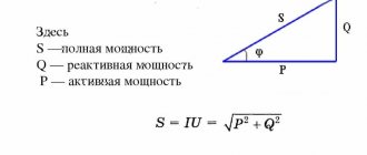
Conditions for transferring maximum power from an energy source to a receiver Let's imagine an energy source with EMF E and internal resistance by an equivalent circuit (Fig. 3.22). Let's find out what the resistance Z=r + jx of the receiver should be so that the active power transmitted to it is maximum. Receiver power Obviously, for any r, the power reaches its greatest value at . In this case, taking the derivative with respect to r from the resulting expression and equating it to zero, we find that P has the greatest value at . Thus, the receiver receives the greatest active power from the source if its complex resistance is conjugate with the complex internal resistance of the source: Under this condition and efficiency In electric power plants, the maximum power transmission mode is unprofitable due to significant energy losses. In various types of automation, electronics and communications devices, the signal powers are very low, so it is often necessary to specially create conditions for transmitting the maximum possible power to the receiver. A decrease in efficiency often does not matter at all, since the transmitted energy is small. Matching the resistances of the receiver and the power source in accordance with (3.50) can also be achieved by adding elements with reactance to the circuit (see example 4.6). Sometimes the resistance of the receiver can be changed without arbitrarily, but only with maintaining the relationship between active and reactance, i.e. at . An analysis, which is not given here, shows that in this case the power P is maximum if the impedances of the receiver and the source () are equal to each other, while matching the impedances of the receiver and the power source can be achieved by turning on the receiver through a transformer. In the general case of a receiver - a branched passive circuit - Z is its input impedance.
See also the section on websor
- Alternating currents
- Concept of alternators
- Sinusoidal current
- Effective current, emf and voltage
- Representation of sinusoidal functions of time by vectors and complex numbers
- Addition of sinusoidal time functions
- Electrical circuit and its diagram
- Current and voltage when connecting resistive, inductive and capacitive elements in series
- Resistance
- Voltage and current phase difference
- Voltage and currents when connecting resistive, inductive and capacitive elements in parallel
- Conductivity
- Passive two-terminal network
- Power
- Powers of resistive, inductive and capacitive elements
- Power balance
- Power signs and direction of energy transfer
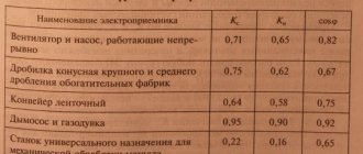
- Determining the parameters of a passive two-terminal network using an ammeter, voltmeter and wattmeter
- Conditions for transferring maximum power from the energy source to the receiver
- Understanding the Surface Effect and the Proximity Effect
- Parameters and equivalent circuits of capacitors
- Parameters and equivalent circuits of inductors and resistors